Tutorial 3: Import XML Purchase Orders Into A Database
This document illustrates mapping into related database tables. The source data will be an XML file, and the destination database will be the same Exo database that we have already worked with, MYOB Exo.
This tutorial represents a case of a supplier receiving electronic purchase orders and automatically processing them into Exo, along with some order validation.
Each step should be fully completed before processing to the next. The topics covered are:
Configuring XML File Definitions to enable the reading of XML files
Configuring the database DB Definitions for writing into related database tables
Using variables in the Statelake Map
Using various events in the Statelake Map
Querying databases from the Map during processing
Control of the execution of the Map, and halting the processing
It is most important before you proceed, to check and ensure that all of the training files have been copied as instructed. These files are an essential part of this tutorial.
XML Files
XML files differ from flat data files because they contain information scattered within the file that relates to the file structure, interspersed with the actual data values. This format tends to make XML files larger in size, but can also make them easier to read.
For example, an order number in an XML file might appear as:
<OrderNumber>12345</OrderNumber>XML also has the advantage of using schema files. These are separate from the data files, and describe the structure of the incoming XML data file, along with any validation rules that each data file must comply with.
The format of these schema files determine how the incoming data is translated and typically have a file name ending with .xsd, whereas XML data files have an .xml file extension.
The following examples show a simple XSD schema file, and the corresponding XML data file.
Simple XML Schema Definition (.XSD) For An Order
<?xml version="1.0"?><xs:schema attributeFormDefault="unqualified" elementFormDefault="qualified" version="1.0" xmlns:xs="http://www.w3.org/2001/XMLSchema"><xs:element name="OrderHeader" type="OrderHeaderType"/><xs:complexType name="OrderHeaderType"> <xs:sequence> <xs:element name="OrderNumber" type="xs:string" minOccurs="1" maxOccurs="1" /> <xs:element name="OrderDate" type="xs:date" minOccurs="1" maxOccurs="1" /> <xs:element name="OrderLine" type="OrderLineType" minOccurs="1" maxOccurs="unbounded" /> </xs:sequence></xs:complexType><xs:complexType name="OrderLineType"> <xs:sequence> <xs:element name="LineNumber" type="xs:int" minOccurs="1" maxOccurs="1" /> <xs:element name="ProductCode" type="xs:string" minOccurs="1" maxOccurs="1" /> <xs:element name="OrderQuantity" type="xs:int" minOccurs="1" maxOccurs="1" /> </xs:sequence></xs:complexType></xs:schema>Simple XML Data File (.XML) For The Same Order
<OrderHeader> <OrderNumber>12345</OrderNumber> <OrderDate>26-10-2011</OrderDate> <OrderLine> <LineNumber>1</LineNumber> <ProductCode>ABC</ProductCode> <OrderQuantity>10</OrderQuantity> </OrderLine> <OrderLine> <LineNumber>2</LineNumber> <ProductCode>XYZ</ProductCode> <OrderQuantity>3</OrderQuantity> </OrderLine></OrderHeader>Where The Data Is - Database Connections
In this tutorial, an Exo database will be used as the destination, so the DB Connection to the Exo database MYOB Exo that has already been established in earlier tutorials can be used, as the information is the same. We do not need to re-create or duplicate it.
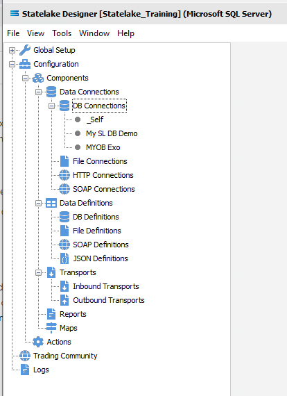
The first step is to make sure that Statelake module Designer for your selected configuration Statelake_Training is open. An expanded structure tree will be displayed on the left side of the screen.
Follow the path Configuration > Components > Data Connections > DB Connections. Click on DB Connections and MYOB Exo should be displayed.
Where The Data Is - File Connections
As we know, the File Connections module also sits under the Data Connections umbrella, and is the configuration module that points to a specified file directory that can hold either or both the source file or destination file. In this tutorial, the output file will be an Exo database, and the source will be a file. So a new file connection for the input/source file needs to be created.
Designer will already be open. If not, open the Statelake module Designer for your selected configuration. An expanded structure tree is displayed on the left side of the screen.
Create File Connection
Follow the path Configuration > Components > Data Connections > File Connections. Right‑click on File Connections and choose New from the drop-down list.
A new item called New File Connection will appear in the structure tree. In the New File Connection window the following information is to be entered.
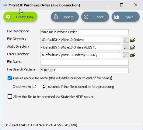
File Description – the name that is meaningful and best describes the file. In this tutorial the description given this connection will be Mitre10: Purchase Order.
File Directory – the directory location of the file. Enter <DefaultDir>\Mitre10 Orders. Use tab to exit the field and move on.
The <DefaultDir> tag refers to the default file path already set-up within Statelake General Setup, under Global Setup. By default, C:\ProgramData\FlowSoftware\Statelake\Files will be the file directory referenced by this tag, and selected.
c. Audit Directory – will be automatically populated when you tab out of File Directory.
d. Error Directory – will be automatically populated when you tab out of File Directory.
Statelake uses two sub-directories to manage files - AUDIT and ERROR. When a file is successfully processed in, or successfully sent after bring written out, it is moved into the AUDIT directory. If an error occurs during file processing, the file is moved into the ERROR directory.
e. File Name – the actual name of the file. In this tutorial, leave this field blank as this connection will not be used to produce any new files – we just want to read from the file.
f. File Search Pattern - used by Statelake when files are being read. Enter M10*.xml to locate all files that match this search criteria. This should locate the three XML files called M10 Order.xml, M10_41919.xml, and M10_41920.xml that are to be used for the source. The asterisk * is a wildcard and replaces any letter in the search. Each of these XML files contain data pertinent to orders.
g. Ensure Unique File Name – tick this box to add a number to the file name to ensure that the file name will be unique and will not overwrite a file already in the output folder.
h. Allow This File To Be Accessed – for this tutorial leave unticked.
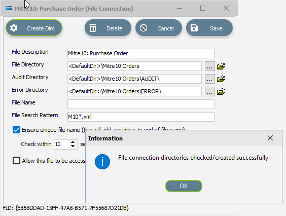
If the sub-directories you have specified do not yet exist or you are not sure whether they exist, you will need to check by clicking on the button Create Dirs which is located on the top left of the window.
If they do not exist, they will be created, else they will be confirmed as current and available by display of the pop-up message “File connection directories checked/created successfully”. Click OK in response to the successful creation message.
Click Save when all details are entered to save and close the module.
The File Connection named Mitre10: Purchase Order will now appear in the structure tree under Configuration > Components > Data Connections > File Connections.
What The Data Is - Creating File Definitions
The File Definitions module is used to design the structure of the files that are either read from, or written to the Statelake configuration. There are four types of files that can be specified in this module - “flat” text files, XML files, Excel (binary), and EDI (EDIFACT) type files. Unlike the flat file that was created in tutorial one, this tutorial uses an XML file as the source. The file is a purchase order file in XML format, and as such the definitions are entered in a different sequence to tutorial one.
EDIFACT is an acronym that stands for Electronic Data Interchange For Administration, Commerce and Transport. It is a more specialised file type that is used in global data transfer, with rules ratified by the U.N.
In this tutorial, a multi-tier XML definition for the input or source purchase orders schema .XSD file and data .XML files will be created.
Designer will already be open. If not, open the Statelake module Designer for the selected configuration. An expanded structure tree is displayed on the left side of the screen.
Create File Definition
Follow the path Configuration > Components > Data Definitions > FIle Definitions. Right‑click on File Definitions and choose New from the drop-down list.
New File Definition will appear as an item in the structure tree. In the New File Definition window the following information is to be entered under the General tab. We will not be accessing the Partner Identification tab during this tutorial.
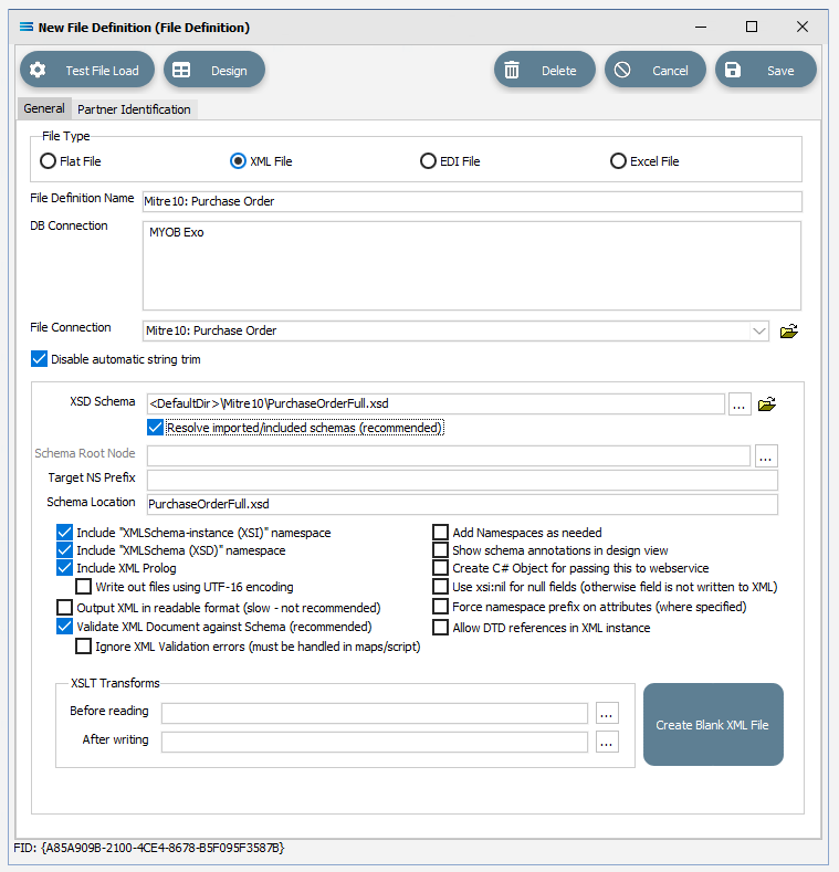
File Type – select XML File.
File Definition Name – the default is New File Definition. Enter the definition name of the source file, as specified during the creation of the File Connection. In this tutorial it is Mitre10: Purchase Order. Make sure that it is typed precisely.
DB Connection – right-click anywhere in the blank DB Connection box to see the Add pop-up, and a list of all the found connections will be displayed by following the arrow. Select the one you want from the list – in this tutorial, it will be MYOB Exo. A source database is required to be selected for all definitions.
If you select the wrong DB Connection, simply double-click on the name within the box to de-select it, and start again.
d. File Connection - select Mitre10: Purchase Order from the pull-down list.
e. Disable Automatic String trim – leave with the default tick as set.
f. XSD Schema – either click the 3-dot ellipse to navigate to the directory where the schema files were copied and select PurchaseOrderFull.xsd by clicking on Open or enter the path name as <DefaultDir>\Mitre10\PurchaseOrderFull.xsd.
When working with XML files, Statelake will always require schema files (XSD), not only to define the structure of the file, but also for validation purposes when reading from, or writing to, an XML file.
g. Resolve Imported/included schemas (recommended) – leave as ticked.
h. All other fields and tick boxes are to be left as defaulted.
Click Design in the top left of the window.
Create File Dataview Query
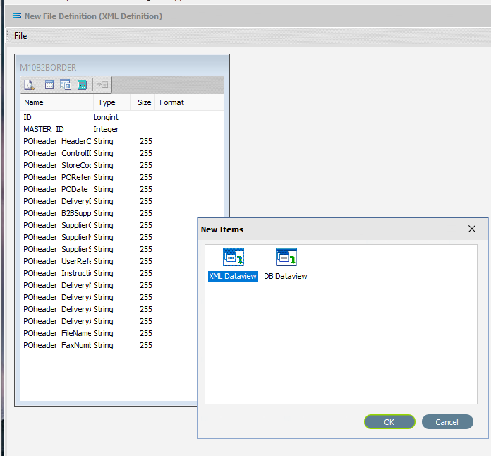
A blank definition designer canvas will display. To start creating the contents of the file definition, click on the File menu in the top left corner, and choose New (or use the Ctrl+N).
The New Items window will open and only two items called XML Dataview and DB Dataview will be displayed.
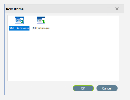
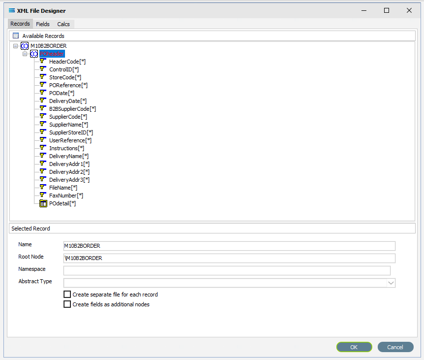
By default, XML Dataview should be highlighted. If not, select XML Dataview and click OK to add a new XML Dataview. The XML File Designer window will open. Expand this window if required, to ensure that the Available Records and Selected Record panes are both displayed fully.
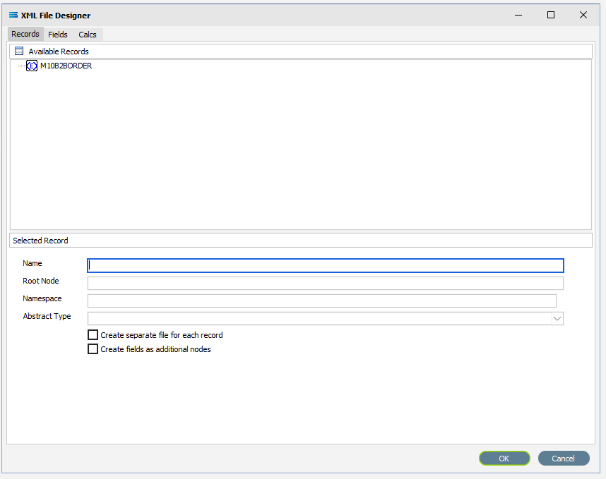
The Records tab will automatically populate some records or elements. There are read from the schema file that you identified on the initial window.
Create M10B2BORDER Root Node
In a tree structure, the Root node is either the topmost or the very bottom branch, depending on how the tree is represented visually. It is the master or starting point – the point from which everything else stems and represents the ultimate objective or main choice. Then there are the Branches, which stem from the root and represent different options, and the Leaf node, which are the last options attached at the end of the Branches.
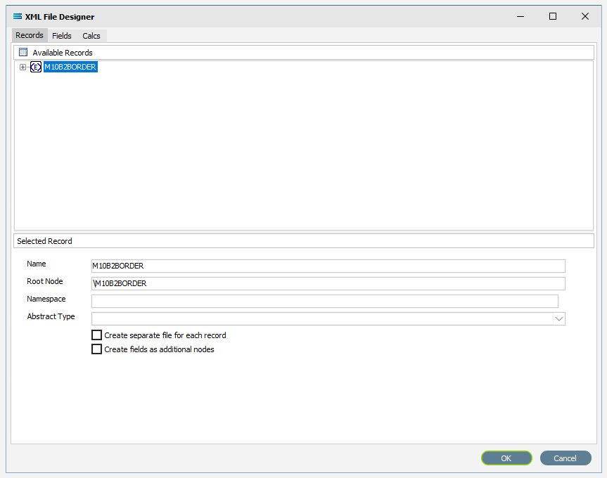
In the XML File Designer window there are three tabs – Records, Fields and Calcs. In this tutorial, the Records tab will display M10B2BORDER in the Available Records pane. If there are multiple entries, scroll down until M10B2BORDER is highlighted and double-click on it to select. M10B2BORDER is the Root Node.
The Name and Root Node fields in the lower Selected Record pane will be automatically populated. M10B2BORDER will appear in the Name field, and \M10B2BORDER will populate the Root Node field.
Root Node in this context is the parent element or file identifier for the group of fields and records that you are adding to this dataview. You will see that the path to the fields will be constructed based on the Root Node you specified.
All other fields and tick boxes are to be left as the set default.
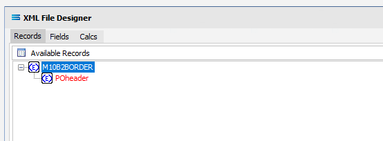
If it has not already been expanded, then click on the plus to expand M10B2BORDER in the Available Records pane.
The structure in the schema file PurchaseOrderFull.xsd determines how these field relationships are handled within this XML File Definition. The top level in the file structure tree is referred to as the Root Node - the name given to the envelope that holds the group of source records. It is the start of the structure tree. In this tutorial, M10B2BORDER is the name given to this group of purchase orders.
The POheader is a node that branches off the Root Node. It is the parent for each XML record and in this tutorial, identifies the fields within each purchase order header. This is a “fat” Branch.
One of the field items in POheader is called POdetail, which is a dataset or group of records in its own right, with its own set of fields, and this is also a Branch - albeit a “twig” off the “fat” Branch. If you wish, you can think of it in this instance, as a Leaf Node. In this tutorial each POheader record can contain multiple POdetail records.
The asterisk (*) at the end of the field name means that you can have more than one of these fields in a single record. There is no limit.
A RED A at the end of the field name identifies the field as an attribute.
There are currently no fields available in the M10B2BORDER root node, but there is a POheader which is displaying in RED because this is a compulsory record.
On the occasion that there are fields under the Root Node itself, they could record information such as who sent the file, when it was sent, and the receiver identity – information that only refers to the file as a whole and is not required more than once. Such fields would be ignored.
There is a symbol to the immediate left of the field name. A BLUE <E> signifies that the item is a non-repeating complex element (a record). A folder icon identifies a repeating complex element (record). A YELLOW T indicates a simple element (a field),
Under Available Records, click on POheader or click the symbol beside it to expand this group (the “fat” Branch), to show the fields within this record grouping. It shows that the header for each record can have multiple fields such as StoreCode and SupplierCode. Expand the window or drag the separator bar between the panes down if required to enlarge the Available Records pane.
The last field in POheader is POdetail which has a series of fields in its’ own right – it is a “twig” or Leaf Node.
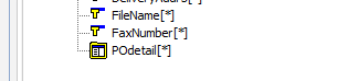
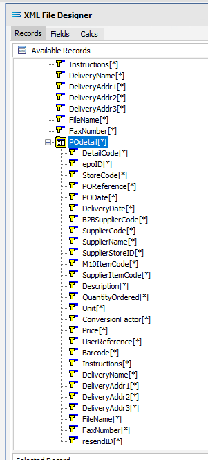
Click on POdetail or click on the symbol beside it to expand it and view the fields under this record grouping. It shows that for each detail field, there can be one or more detail lines that has its own series of fields. Scroll up and down to see them all if required.
Move to the Fields tab in the Available Fields pane and all the fields grouped under POheader and POdetail will be displayed in the upper Available Fields pane.
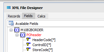
While POheader and POdetail appear in the Available Fields list, they are simply the name or identifying label for the group of fields within them, and are to be treated as such and are to be ignored for selection. With the exception of the group label POheader and POdetail, add all of the fields from the POheader element only by double‑clicking on each field in turn. Once selected they will appear in the Selected Fields pane, showing the data type, length, and XPath of each selected field. As you select the fields, they do not disappear from the Available Fields list.
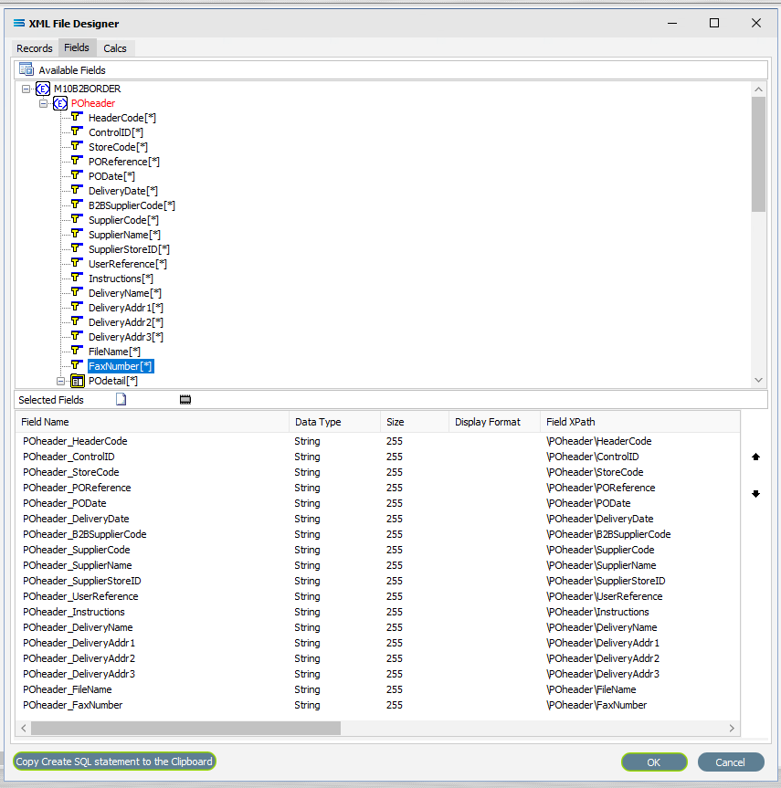
The first field should be POheader_HeaderCode, and the final field to be selected should be POheader_FaxNumber. Expanding the window will only expand the Available Fields pane. In the Selected Fields pane, all fields will be prefixed with POheader_ (the word POheader and an underscore) to identify the original record.
If you want to select two instances of the same field, click on the field name in the Available Fields pane for each instance. The second and subsequent selections will appear in the Selected Fields pane with a sequential number appended to the end of the field name.
If you make a mistake and click on one of the fields in the Available Fields pane that you do not actually require, or click on a field more than once in error, to de-select it, simply double-click on the field name in the Selected Fields pane that you do not want.
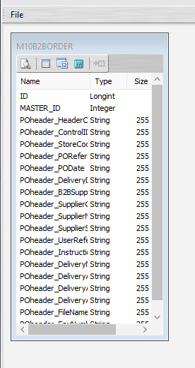
Click the OK button to save and close the window. You will return to the Mitre10: Purchase Order (XML Definition) canvas and a definition window named M10B2BORDER will be visible identifying those fields only contained within POheader. Expand the window as required.
The folder icon that was visible beside POdetail on the previous screen showed that this item was repeating within the header record – meaning that there were multiple detail records for each header record. Therefore, it is treated as a node in its own right and in Statelake, will be shown as an “expanded” Root Node. Create another XML Dataview for this node POdetail by clicking on the File menu in the top left corner, and choose New (or use the Ctrl+N).
The New Items window will open and again, only two items called XML Dataview and DB Dataview will be displayed. Select XML Dataview and click OK to add a new XML Dataview.
Create PODETAIL Root Node
The XML File Designer window will open the Records tab and display M10B2BORDER with the expanded POheader and POdetail fields in the Available Records pane. POheader will appear in RED.
If the fields are not expanded, then double-click on M10B2BORDER to select and expand the records list. Scroll down to POdetail then double-click on it to select it, and populate the Selected Record pane.
The Name and Root Node fields in the lower Selected Record pane will be automatically populated. The Name will now say PODETAIL. The Root Node will now say \M10B2BORDER\POheader\POdetail. This signifies that the Root Node called POdetail is off POheader and within the M10B2BORDER envelope.
All other fields and tick boxes are to be left as the set default.
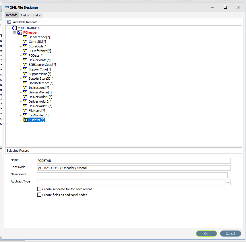
If it is not already expanded, either click on the plus or double-click on POdetail to expand this group and show the fields within this record grouping. Make sure the Name and Root Node do not change.
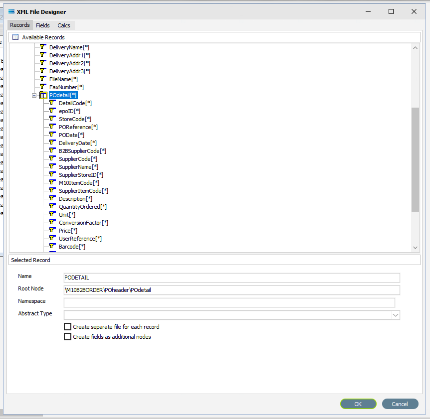
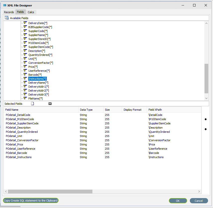
Move to the Fields tab, and all the fields grouped under POdetail will be displayed in the upper Available Fields pane.
For this tutorial, not all detail fields are required to be selected. Add the following fields to the Selected Fields pane only by double‑clicking on them in the Available Fields pane:
DetailCode
M10ItemCode
SupplierItemCode
Description
QuantityOrdered
Unit
ConversionFactor
Price
UserReference
Barcode
Instructions
In the Selected Fields pane, all fields will be prefixed with POdetail_ (the word POdetail and an underscore) to identify the original record.
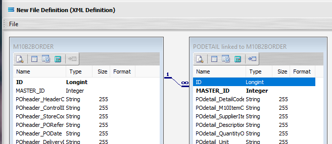
Click on OK to save and close the window. You will return to the Mitre10: Purchase Order (XML Definition) canvas and now there will be two definitions – one named M10B2BORDER showing the fields from POheader, and one named PODETAIL showing the selected fields from POdetail. Expand these windows as required.
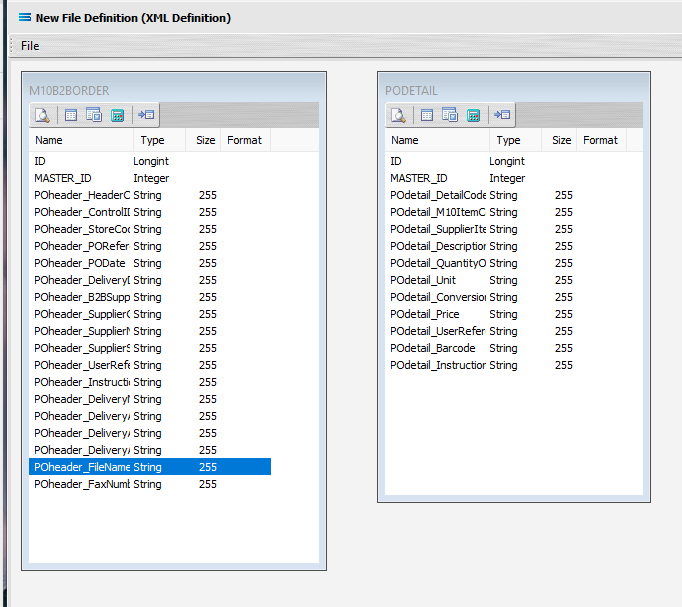
The extra fields ID and MASTER_ID in the dataview are automatically generated by Statelake to enhance the building of the file relationships, and are not included in the mapping process.
Link The Datasets
To link the two together (M10B2BORDER and PODETAIL), we add a relationship between the two datasets by dragging the MASTER_ID field from the PODETAIL dataview containing the fields from POdetail, and dropping it onto the ID field of the dataview M10B2BORDER containing the fields from POheader. Click on PODETAIL_MASTER_ID, drag it so that the label shows as per the example, then unclick to drop it.
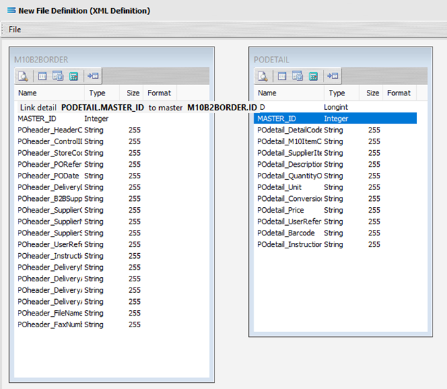
Three things will happen. PODETAIL will be renamed to PODETAIL linked to M10B2BORDER. A one‑to‑many relationship link symbol will appear between the two dataviews - the one “single” link pointing at ID in M10B2BORDER, and the many pointing at MASTER_ID in the renamed dataview PODETAIL linked to M10B2BORDER. And ID in M10B2BORDER will be bolded, as will MASTER_ID in PODETAIL. The line of the link indicator will appear at the top of the item it is linked it.
The links between the two datasets have now been successfully completed. Columns and window borders can be resized as required by dragging them with the mouse. Close the definition canvas by selecting Close from the File menu. You will return to the File Definition window. Click Save to save and close the New File Definition module. Always remember to select Save here – else all of your hard work linking these datasets will not be saved.
To ensure that the mapping will work as it should it is important to do a double check to make sure that your File Definitions are correct, and the parent/child relationship is described as it needs to be.
You can re-open the File Definition called Mitre10:Purchase Order, and click Design on the opening window. This takes you to the canvas where M10B2BORDER and PODETAIL linked to M10B2BORDER are displayed, along with their field link. Click on the Records tab on each dataset in turn to bring up the XML File Designer window for the respective dataset.
For M10B2BORDER - ensure that the Name is M10B2BORDER and the Root Node is \M10B2BORDER. Cancel to exit the window.
For PODETAIL - ensure that the Name is PODETAIL and the Root Node is \M10B2BORDER\POheader\POdetail. Cancel to exit the window.
If this is not correct, you will need to return to the previous three sections Create M10B2BORDER Root Node, Create PODETAIL Root Node, and Link The Datasets and do them again.
Then select File followed by Close to exit the canvas, then Cancel to exit the File Definition window.
The File Definition named Mitre10: Purchase Order will now appear in the structure tree under Configuration > Components > Data Definitions > File Definitions.
You have now successfully created a file definition for an XML file type with a multi‑tier dataset.
What The Data Is - Creating DB Definitions
The DB Definition tells Statelake what the data is, so that the proper fields can be accessed and the data extracted correctly, which means defining the exact information to be extracted. The DB Definition also identifies how the output file is to be constructed.
Sitting under the Data Definitions umbrella, Statelake uses the DB Definitions module to define these data structure components, and to design the database queries for both reading the data out of, and writing in to, the databases. Illustrating the subtle but important differences with this type of destination definition, this tutorial uses two related tables for the output, or destination.
Designer will already be open. If not, open the Statelake module Designer for the selected configuration. An expanded structure tree is displayed on the left side of the screen.
Create DB Definition
Follow the path Configuration > Components > Data Definitions > DB Definitions. Right‑click on DB Definitions and choose New from the drop-down list.
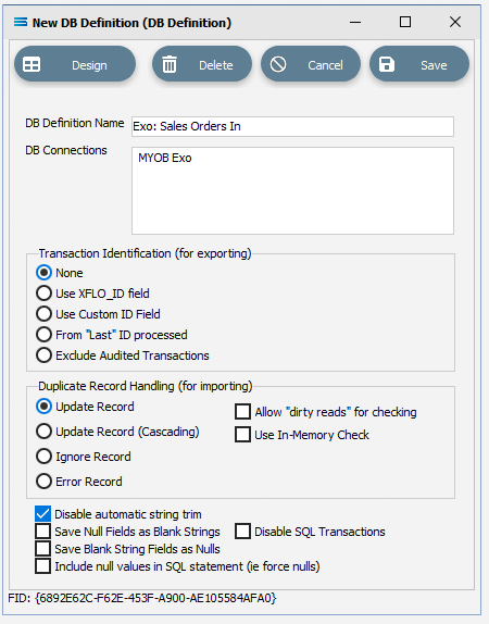
The item New DB Definition will appear in the tree. In the New DB Definition window the following information is to be entered.
DB. . Definition Name – the name that is meaningful and best describes the query/extraction. We will use Exo: Sales Orders In.
DB Connections – this is the name of the source database, identified by the meaningful name that was given in the DB Connections module. Right-click anywhere in the box to see the Add pop-up, and a list of all the found connections will be displayed. Follow the arrow and select the one you want from the list – in this tutorial, it will be MYOB Exo.
Remember, that if you select the incorrect DB Connection, simply double-click on the DB Connection name within the box to de-select it and start again. It is very easy to correct.
c. Transaction Identification – leave with the defaults as set.
d. Duplicate Record Handling – leave with the defaults as set.
e. Disable Automatic String Trim – leave with the default as set. This box is ticked.
f. Save Null Fields as Blank Strings – leave with the default as set.
g. Disable SQL Transactions – leave with the default as set.
h. Save Blank String Fields as Nulls – leave with the default as set.
i. Include Null Values in SQL statement – leave with the default as set.
Click Design in the top left of the window.
Create 1st DB Dataview Query
A blank definition designer canvas will display. To start creating your query, click on the File menu in the top left corner, and choose New (or use the Ctrl+N).
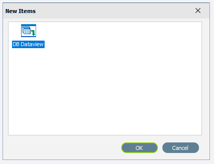
The New Items window will open and only one item called DB Dataview will be displayed. Click OK to add DB Dataview.
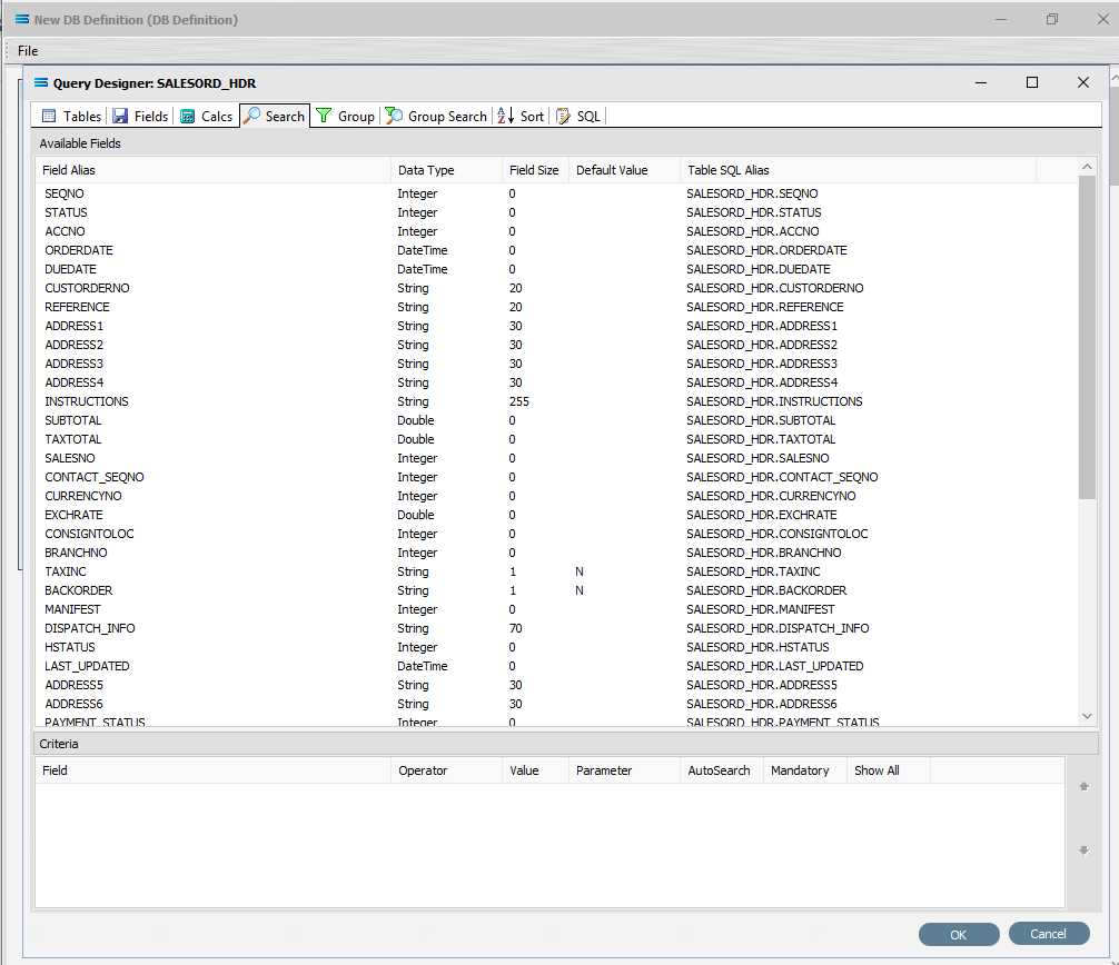
The Query Designer window will open.
The first tab in the Query Designer is Tables. The upper pane contains a list of available tables in alphabetic order, and the lower pane will display the tables that you have selected during this process. Scroll down the available tables to SALESORD_HDR (Sales Order Header) and double-click to select it. It will appear in the lower pane as a selected table, while still remaining visible in the upper pane.
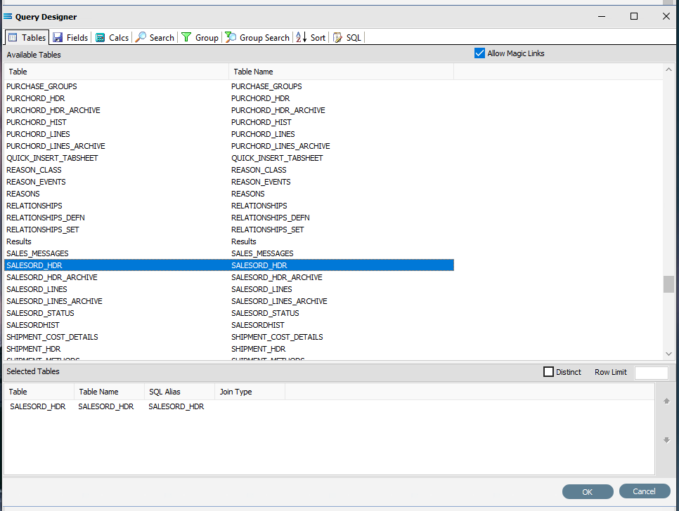
You may have to expand the window height to see a greater number of entries.
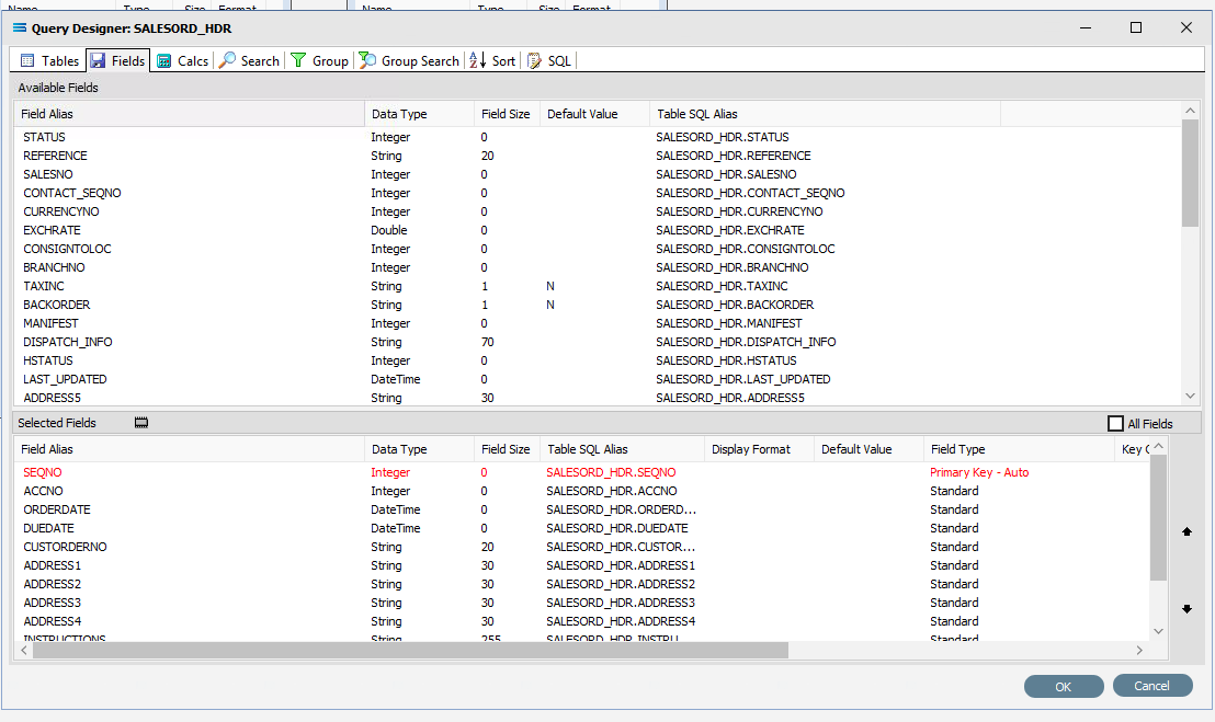
Move to the Fields tab, and add the following fields to query by double-clicking on them. As each one is selected, it will disappear from the upper pane and appear in the lower pane. SEQNO will be displayed in RED.
If you make a mistake and select the wrong field, then simply double-click on it in the lower pane and it will de-select and reappear in the upper pane.
SEQNO (sequence number)
ACCNO
ORDERDATE
DUEDATE
CUSTORDERNO
ADDRESS1
ADDRESS2
ADDRESS3
ADDRESS4
INSTRUCTIONS
SUBTOTAL
TAXTOTAL
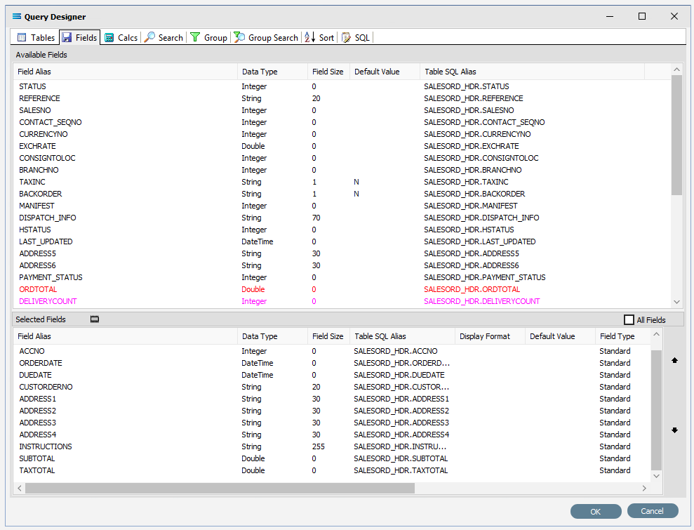
The fields are colour coded in the Query Designer. RED indicates that the field is either calculated or it is an automatically generated IDENTITY type, such as SEQNO. PINK indicates that the field does not allow null values.
Click on the SQL tab to see the SQL query that has been generated. It lists the fields you selected and the table they are to be retrieved from. You will see that each field is prefixed with the table name with a full-stop as a separator.
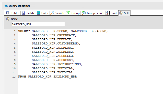
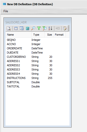
Click OK at the bottom-right of the Query Designer to save the dataview and return to the definition canvas. The configured dataview will display, listing all of the selected fields. Expand this window as required.
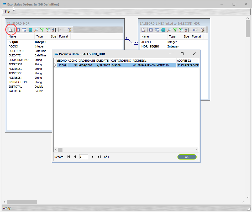
Click on the Preview button to run the query and see the results which will open in a specific window called Preview Data – SALESORD_HDR.
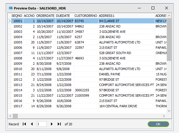
Click OK at the bottom of the preview window to return to the definition canvas and the open dataview.
Create 2nd DB Dataview Query
Create another DB Dataview by clicking on the File menu in the top left corner, and choose New (or use the Ctrl+N).
The New Items window will open and only one item called DB Dataview will be displayed. Click OK to add DB Dataview.
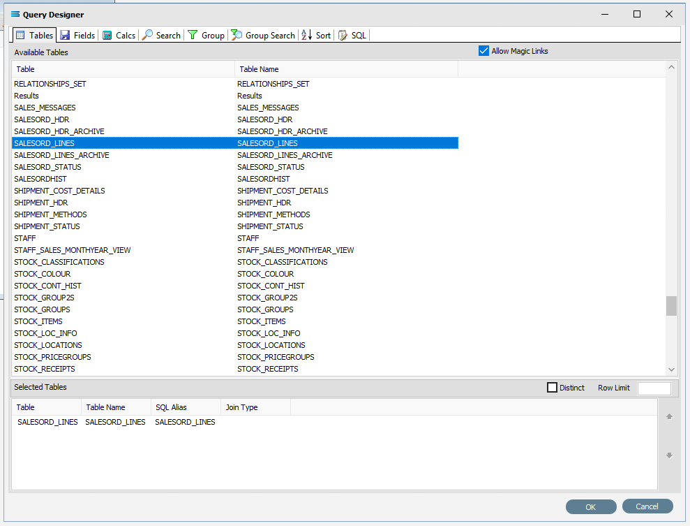
13. The Query Designer window will open on the Tables tab. The upper pane contains a list of available tables in alphabetic order, and the lower pane will display selected tables. Scroll down the available tables to SALESORD_LINES (Sales Order Lines) and just as we did for the SALESORD_HDR table, double-click on the SALESORD_LINES table to select it, and it will appear in the lower pane as a selected table.
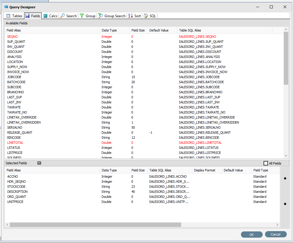
Move to the Fields tab, and add the following fields to query by double-clicking on them:
ACCNO
HDR_SEQNO (order header sequence number)
STOCKCODE
DESCRIPTION
ORD_QUANT
UNITPRICE
As you select fields from the Available Fields pane, they will appear in the Selected Fields pane, and disappear from the Available Fields pane.
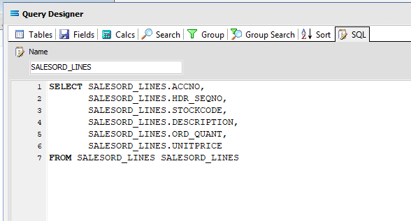
You can click on the SQL tab to see the SQL query that has been generated. It lists all of the fields you selected and the table they are to be retrieved from.
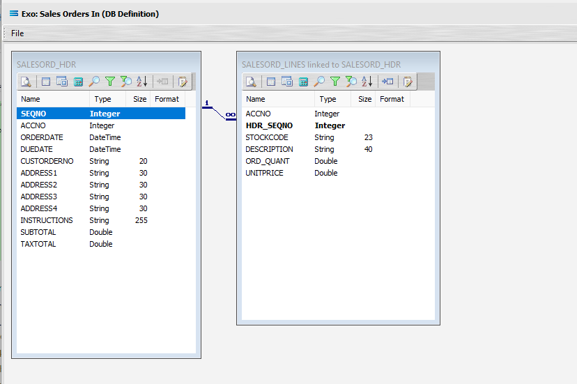
Click OK at the bottom-right of the Query Designer to save the dataview and return to the definition canvas. The configured dataview will display, listing all of the selected fields, so now there will be two definitions visible on the canvas - one named SALESORD_HDR and one named SALESORD_LINES. Expand the windows as required.
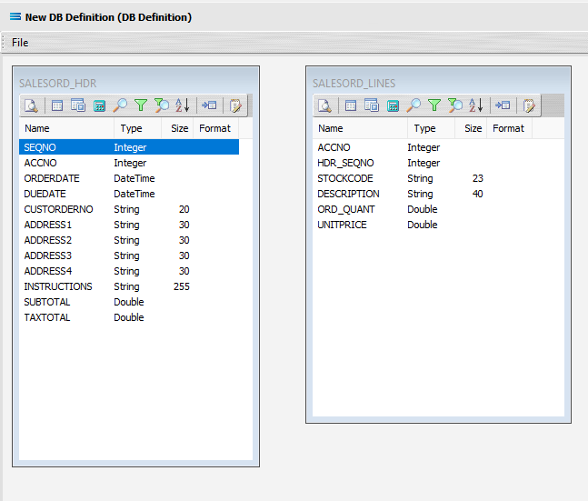
Link The Datasets
We want to link these together, so add a relationship between the two datasets by dragging the HDR_SEQNO field from the SALESORD_LINES dataview and dropping it onto the SEQNO field of the dataview SALESORD_HDR. Click on SALESORD_LINES.HDR_SEQNO and drag it over to SALESORD_HDR.SEQNO - once you see the drag label as below, then unclick to drop it.
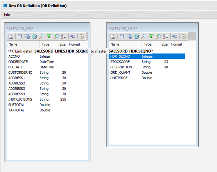
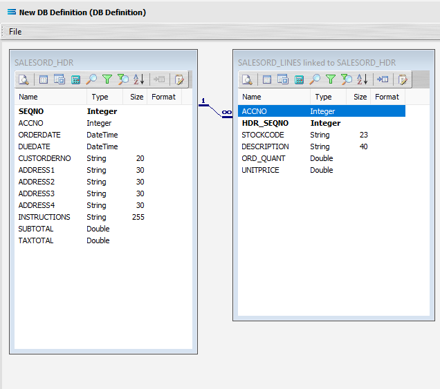
Three things will happen. SALESORD_HDR will be renamed to SALESORD_LINES linked to SALESORD_HDR. A one-to-many relationship link will appear between the two dataviews - the “single” link pointing at SEQNO in SALESORD_HDR, and the many pointing at HDR_SEQNO in the renamed dataview SALESORD_LINES linked to SALESORD_HDR. These two linked fields will also be bolded.
Now we want to add some criteria. Either, click the Search tab on the SALESORD_HDR dataview to open the Query Designer window on the Search tab, or get to the same place by simply clicking on the Tables tab for the dataview, and when the Query Designer window opens, move to the Search tab. Expand the window as required.
The upper pane shows the Available Fields, under the heading of Field Alias. Double-click on SEQNO in this list (SALESORD_HDR), and the field name will appear in Criteria pane. The field name will not disappear from the top pane once selected. To remove a field selected in error, simply double‑click on it in the Criteria pane to de-select.
To change the sort sequence of the field name list, click on the Field Alias column name to toggle the sequence. Click once to sort alphabetically from in descending order from A - Z; click again to toggle to ascending order from Z - A; click again to return to the default sequence (as per the table design).
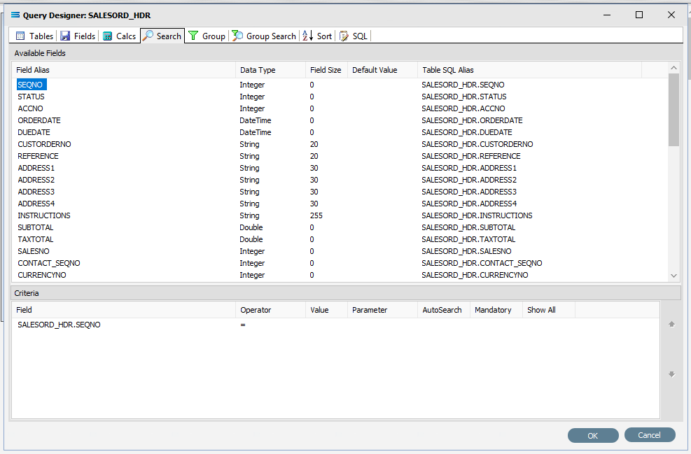
To the right of the field name in the Criteria pane, several extra fields will appear, including Operator and Value. Leave the Operator as defaulted as an equal sign (=), and enter -1 as the Value, to ensure that the DB Definition is empty when it is loaded into the map. If this dataset holds any data, then Statelake will produce an error, so to successfully insert or update data into a populated table, the search criteria is set to a value that will not exist in the table (such as -1), Tab out of the Value field.
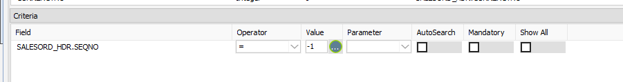
Statelake will generate an error during the start of mapping if the destination dataset contains any data prior to the operation. So entering a value if minus 1 (-1) into the value field forces the destination dataset to be completely empty of any residual data.
Now leave the Search tab and move left into the Fields tab. Under Selected Fields, under the Field Type column, all the fields that you selected earlier will be displayed and all will have a Field Type of Standard. SEQNO will be displayed in RED.
Change the Field Type on SEQNO to Primary Key – Auto, by clicking on the Field Type for the line and selecting this option from the pull-down list. If Primary Key – Auto does not display properly, then expand the width of the column. Primary Key - Auto should be first at the top of the list.
Selecting Primary Key - Auto identifies this field SEQNO as a field that will have its values automatically generated by the database server in the SALESORD_HDR dataset. This means that when a header record is written to SALESORD_HDR, a value will automatically be assigned to the SEQNO column/field. This SEQNO value is then written into the related line records into the HDR_SEQNO field in the SALESORD_LINES dataset, keeping the link between the two datasets accurate and well defined.
Click on the empty Key Generation column for this field to see the pull-down list of available values. If the column does not seem to populate, make sure that you have selected SEQNO and that the column fields are bordered. Select SELECT SCOPE_IDENTITY(). This option should be at the top of the list.
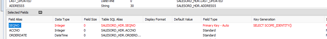
Using this as the Key Generation means that the system will keep a track of the last identity value that was accessed by this particular session query. This keeps the child records correctly linked to the appropriate parent record.
If the column width default for Field Type and Key Generation are too small to see the full options, expand the columns as required with the mouse.
Click OK at the bottom-right of the Query Designer to save the dataview and return to the definition canvas.
Now, either click the Tables tab on the SALESORD_LINES linked to SALESORD_HDR dataview, and in the Query Designer window click on the Fields tab. Or, click on the Fields tab on the same table.
In the Selected Fields pane, set the Field Type on the HDR_SEQNO field to Foreign Key. The HDR_SEQNO Field Type is set to Foreign Key because the field is related to SEQNO from the SALESORD_HDR dataset, and with this setting Statelake will automatically assign the SALESORD_HDR SEQNO value to this field.

Click OK at the bottom-right of the Query Designer to save the dataview and return to the definition canvas.
Close the definition canvas by selecting Close from the File menu. You will return to the EXO: Sales Orders In window.
Click Save to save and close the module.
The DB Definition named EXO: Sales Orders In will now appear in the structure tree under Configuration > Components > Data Definitions > DB Definitions.
What To Do With The Data - Creating Maps
There have now been two definitions created for this tutorial – the File Definition called Mitre10: Purchase Order, and the DB Definition called Exo: Sales Orders In.
Designer will already be open. If not, open the Statelake module Designer for the selected configuration. An expanded structure tree is displayed on the left side of the screen.
Create The Map
Follow the path Configuration > Components > Maps. Right‑click on Maps and choose New from the drop‑down list.
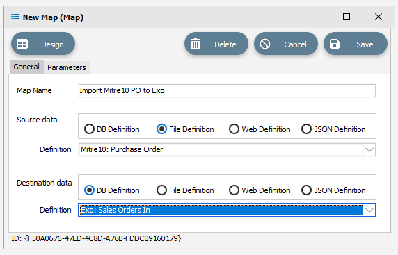
New Map will appear as an item on the tree. The New Map window contains two tabs - General and Parameters. The Parameters tab allows you to set other options, but for training purposes, we will be dealing with just the General tab. The following information is to be entered for the main map.
Map Name - this is the meaningful name that will identify the extraction process, and in this tutorial will be called Import Mitre10 PO to Exo.
Source Data – highlight the File Definition radio button.
Definition – the File Definition that was created for this configuration called Mitre10: Purchase Order can be selected from the pull-down list.
Destination Data – highlight the DB Definition radio button.
Definition – the name of the DB Definition that was created for this configuration called EXO: Sales Orders In can be selected from the pull-down list.
Open The Map
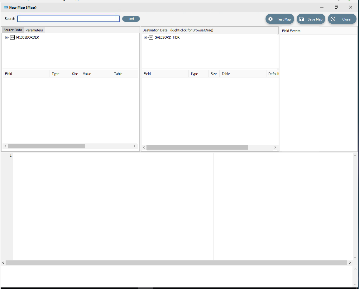
Click the Design button in the top left of the window to open the map designer window New Map.
The New Map screen is split into five distinct panes beneath the search bar.
Source is split into two panes with Source Data and Parameters tabs. This is the definition of the source that data is to be read from.
Destination Data is also split into two panes. This is the definition that the data is to be written to.
Field Events on the right side of the screen. The events of the selected dataset or record.
Scripting Area beneath the Source and Destination Data panes. Where the script of each event is displayed and edited.
Compiler Messages below the Scripting Area. Messages that are returned by the compiler.
The first mapping operation is the linking of the datasets, to ensure that for every record in the source dataset there is a corresponding record in the destination dataset.
In this tutorial we will link the source dataset table M10B2BORDER to the destination SALESORD_HDR dataset. M10B2BORDER is already showing in the Source Data pane, and SALESORD_HDR is already showing in the Destination Data pane.
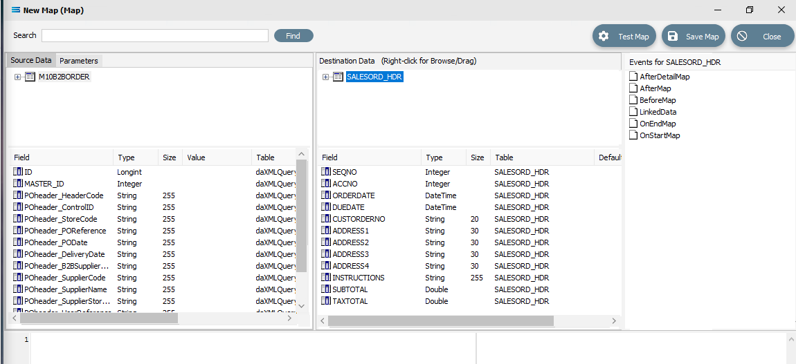
If you click on M10B2BORDER in the Source pane you will see the field names that are in the XML file appear in the lower part of the pane. Expand the pane if required.
If you click on SALESORD_HDR in the Destination Data pane, the fields in this dataset will appear in the lower part of the pane.
Link The Datasets And Populate The Map
Link the two by dragging the XML Root Node called M10B2BORDER and dropping it onto the SALESORD_HDR dataset. You will see the established link appear in the Scripting Area, where the LinkedDataEvent code has been automatically generated.
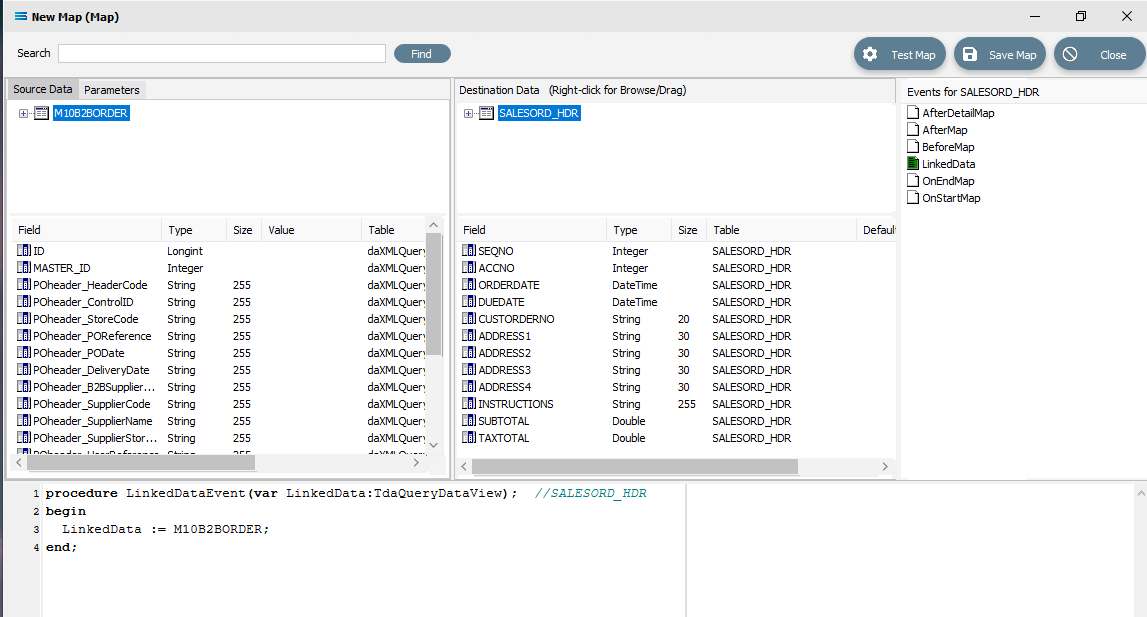 Close up of the script.
procedureLinkedDataEvent(varLinkedData:TdaQueryDataView);// SALESORD_HDRbeginLinkedData := M10B2BORDER;end;A list of events has also appeared in the Field Events pane, and this has been renamed to Events For SALESORD_HDR. The file icon beside the LinkedData event is now coloured GREEN which indicates a successful compilation for this event. If the icon was RED, this would indicate that the code was not successfully compiled.
Double-click on M10B2BORDER in the Source Data pane to display the linked node PODETAIL. Double‑click on SALESORD_HDR in the Destination Data pane to display the linked database table SALESORD_LINES.
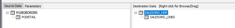
Link these two by dragging the PODETAIL node and dropping it onto the SALESORD_LINES database table. You will see the established link appear in the Scripting Area, where the LinkedDataEvent code has been automatically generated.
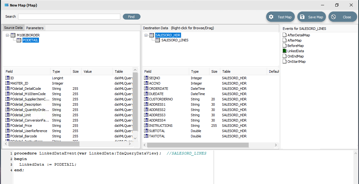 Close up of the scripting.
procedureLinkedDataEvent(varLinkedData:TdaQueryDataView);// SALESORD_LINESbeginLinkedData := PODETAIL;end;A list of events has also appeared in the Field Events pane, and this has been renamed to Events For SALESORD_LINES. The file icon beside the LinkedData event is now coloured GREEN.
Link The fields
Click on SALESORD_HDR in the Destination Data pane. Then click on ACCNO in the Field list in the lower pane. Set the ACCNO field value manually to 1. Do this by clicking anywhere in the Scripting Area panel and Statelake will generate code. Append to the third line and type 1 immediately after the Value :=.
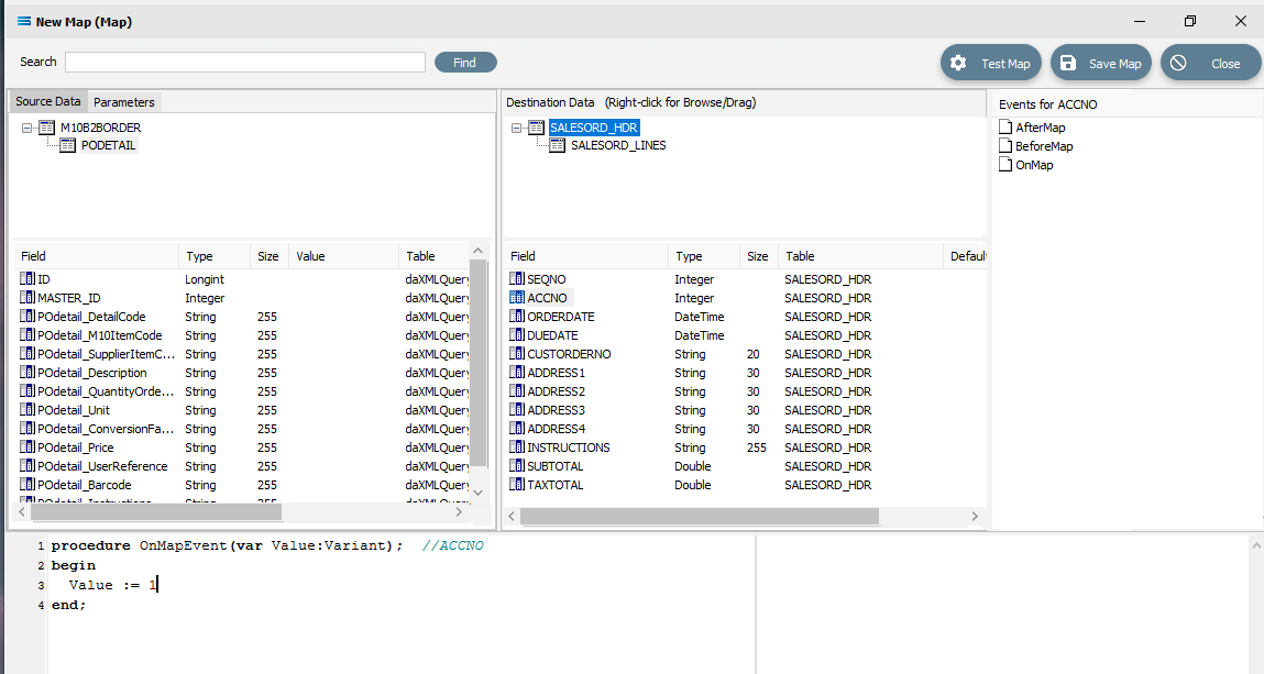 Close up of the script.
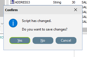
procedureOnMapEvent(varValue:variant);// ACCNObeginValue :=1end;When you click on another field name in the Destination pane, you will be prompted to save your changes. Click Yes.
ACCNO has now changed to GREEN. Now link the fields using the same drag and drop technique used previously - drag the fields from the Source Data M10B2BORDER and drop onto the Destination Data field belonging to SALESORD_HDR, making sure that the destination field is highlighted before dropping the source field onto it, else the link will not be successfully established. Click on M10B2BORDER and SALESORD_HDR to bring up the correct series of fields, then drag and drop -
POheader_PODate to ORDERDATE
POheader_DeliveryDate to DUEDATE
POheader_POReference to CUSTORDERNO
POheader_DeliveryName to ADDRESS1
POheader_DeliveryAddr1 to ADDRESS2
POheader_DeliveryAddr2 to ADDRESS3
POheader_DeliveryAddr3 to ADDRESS4
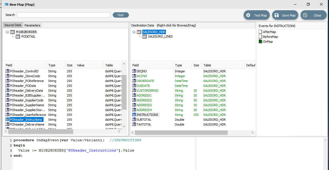
POheader_Instructions to INSTRUCTIONS
For each successful field drop, the colour of the field name in the Destination Data pane changes to GREEN, and an OnMapEvent procedure appears in the Scripting Area. In the Field Events pane, a set of events for each field has appeared, and each successful link is indicated by the OnMap event file icon being shown in GREEN.
The SALESORD_HDR.SUBTOTAL and SALESORD_HDR.TAXTOTAL fields are not populated through this drag-and-drop process. They need to be manually set to 0 (zero) as these totals are not given in the source file and need to be calculated. Click on the SUBTOTAL field in the lower destination pane, then click anywhere in the Scripting Area panel to generate the code. Append to the third line and type 0 (zero) immediately after the Value :=.
procedureOnMapEvent(varValue:Variant);//SUBTOTALbeginValue :=0end;When you click out of the Scripting Area onto the SALESORD_HDR.SUBTOTAL field or another SALESORD_HDR field, you will be prompted to save your changes. Click Yes.
Now click on the TAXTOTAL field and repeat the process, appending a 0 (zero) to the Value := line.
procedureOnMapEvent(varValue:Variant);//TAXTOTALbeginValue :=0end;And again, when you click out of the Scripting Area onto the SALESORD_HDR.SUBTOTAL field or another SALESORD_HDR field, you will be prompted to save your changes. Click Yes.
Now that the mapping of SALESORD_HDR is complete, the fields in SALESORD_LINES need to be mapped as well. Click on PODETAIL in the Source Data pane to bring up the associated fields in the lower Source Data pane, and then click on SALESORD_LINES in the upper Destination Data pane to bring up the relevant fields in the lower pane.
The value for SALESORD_HDR .SEQNO will be automatically generated by the Statelake process, and SALESORD_LINES.HDR_SEQNO is set as a Foreign Key in the DB Definition, so the value will be automatically populated from the linked related field from SALESORD_HDR.
The following remaining fields will be linked by the drag-and-drop process. Each successful drop will generate some script and the Destination Data pane field names will change to GREEN.
POdetail_SupplierItemCode to STOCKCODE
POdetail_Description to DESCRIPTION
POdetail_QuantityOrdered to ORD_QUANT
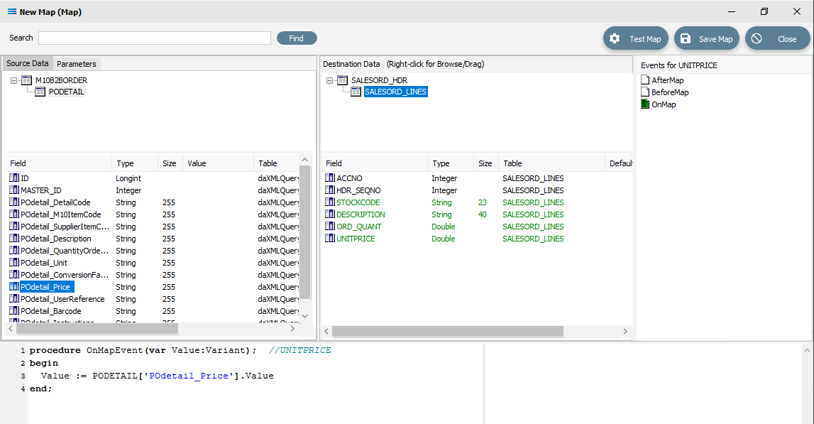
POdetail_Price to UNITPRICE
In the destination fields pane, click on ORD_QUANT, and change the end of line 3 of the script from .Value to .AsFloat to force a data type conversion.
procedureOnMapEvent(varValue:Variant);//ORD_QUANTbeginValue := PODETAIL['POdetail_QuantityOrdered'].AsFloatend;Then click on SALESORD_LINES.UNITPRICE, and you will be prompted to save your changes. Click Yes.
Now that UNITPRICE is selected, change the end of line 3 of the script from .Value to .AsFloat to force a data type conversion.
procedureOnMapEvent(varValue:Variant);//UNITPRICEbeginValue := PODETAIL['POdetail_Price'].AsFloatend;Click on another field such as UNITPRICE, and you will be prompted to save your changes. Click Yes.
Create Detailed Scripts
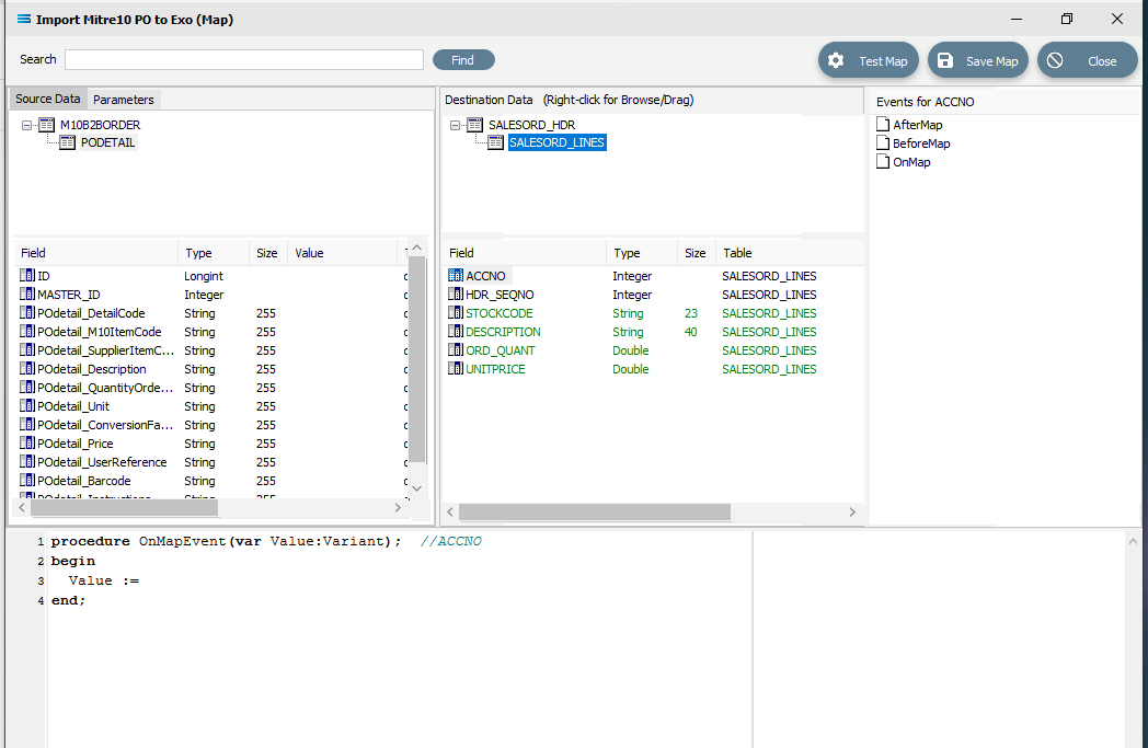
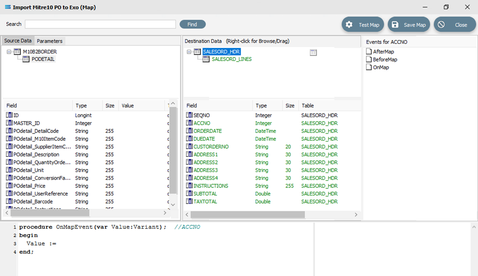
Although the value for SALESORD_LINES.ACCNO is already specified on SALESORD_HDR, the mapping script for this field needs to be manually set. With the SALESORD_LINES dataset selected and its fields displayed, click on ACCNO. The digit 1 will appear in the Scripting Area.
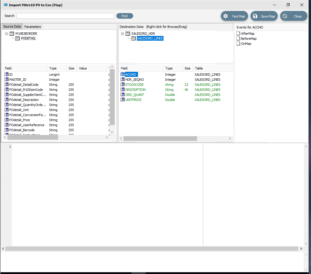
Click anywhere in the Scripting Area to generate the base code.
If this “empty” base code fails to generate and just the number 1 continues to be displayed, go to the Events for ACCNO pane in the top right of the window, and right-click on the GREEN OnMap icon - the icon itself, not the words OnMap. Select Clear from the pop-up. This will reset the script window so that you can try loading the base script again by clicking anywhere within the scripting window while SALESORD_LINES.ACCNO is selected in the destination pane.
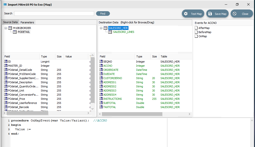
With this code still active, we need to swap over control to access the field name in SALESORD_HDR. To achieve this, follow these steps – be aware, it is easy to lose track of where you are!
The dataset SALESORD_LINES in the Destination Data pane should still be highlighted. RIGHT-click on SALESORD_HDR in the Destination Data pane to give control over to this dataset. You should get the cursor to change to a diagonally-barred circle. The relevant fields belong to this dataset will appear in the lower pane.
Now LEFT-click with your cursor in the blank space in the top right hand side of the top Destination Data pane. A right-click would usually copy and a left-click will normally paste. But as we are using this right‑click to simply swap datasets, the copy/paste is not required. You will see that the Scripting Area still displays the code that we generated for the ACCNO field in SALESORD_LINES - the code does not change.
But now we do want to copy/paste, so RIGHT-click on SALESORD_HDR.ACCNO as is displayed in the lower portion of the Destination Data pane to copy the field name. You should get the cursor to change to a diagonally-barred circle beside ACCNO.
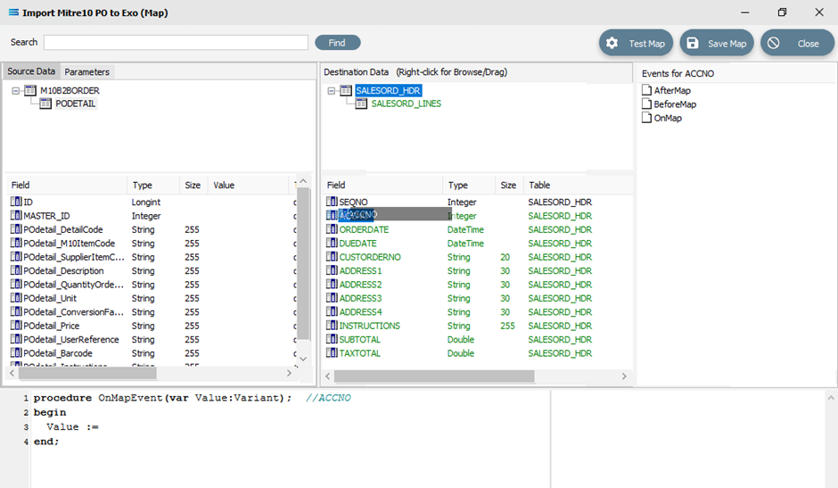
Then left-click with your cursor in the Scripting Area at the end of the 3rd line to append the field name to the Value := to post/append this code to the end of the line.
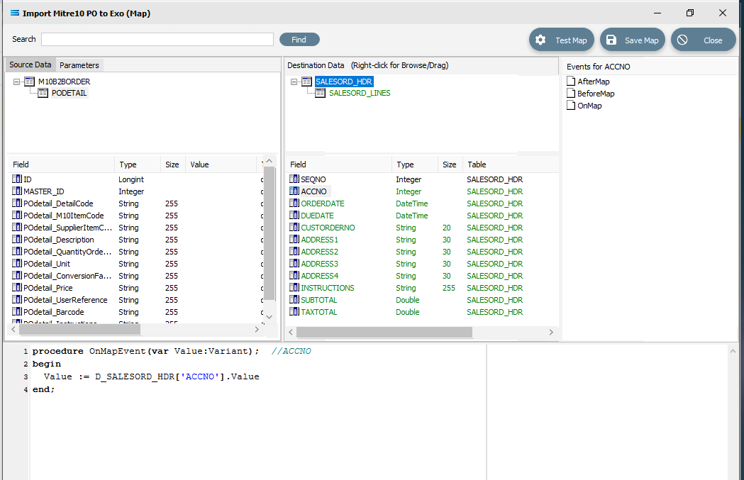
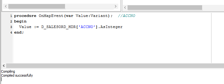
The code should now be as below. The D_ denotes that the field is from a destination dataset. A close up of the code follows.
procedure OnMapEvent(var Value:Variant); //ACCNObegin Value := D_SALESORD_HDR['ACCNO'].Valueend;The line needs one further amendment. The .Value at the end of the line that you have just pasted, needs to be replaced by .AsInteger, so the code matches the example below.
procedure OnMapEvent(var Value:Variant); //ACCNObegin Value := D_SALESORD_HDR['ACCNO'].AsIntegerend;Click anywhere in the Scripting Area pane to select Test Compile and check that the code is correct.
To verify that this code applies to ACCNO in SALESORD_LINES, click on the SALESORD_LINES dataset. You will be prompted to save your script changes – click Yes. Then click on the field ACCNO. This field should now display in GREEN and the compiler area should show that the code has been successfully compiled. If the compile fails, check your spelling and try again.
There are two fields in SALESORD_HDR that need further modifications to their script code. ORDERDATE and DUEDATE are presented as strings in the input/source dataset, but as the destination/output stores these valuesneed to be proper dates, so these strings need to be converted into the DateTime data type using the StringToDateTime function. Click on SALESORD_HDR to load the fields into the lower pane.
Click on ORDERDATE to display the OnMapEvent code in the Scripting Area. We want to change line 3 of the code from Value := M10B2BORDER['POheader_PODate'].Value to the following code.
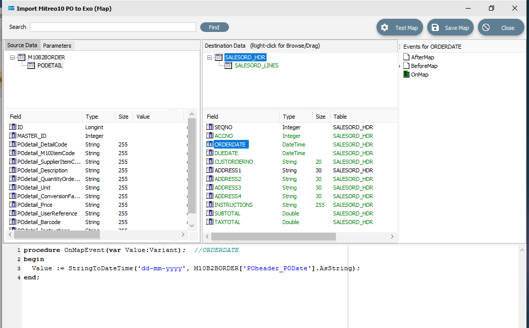 Close up of the code follows.
procedure OnMapEvent(var Value:Variant); //ORDERDATEbegin Value := StringToDateTime('dd-mmm-yyyy', M10B2BORDER['POheader_PODate'].AsString);end;When you click out of the Scripting Area, if you are prompted to save your changes, click Yes. This field should now display in GREEN.
To test your scripting to ensure that it holds no errors and will compile successfully, you can right-click in the blank space of the scripting area and select Test Compile from the list.
Click on DUEDATE to display the code in the Scripting Area. Change line 3 in the script in the same manner, so as it reads as below.
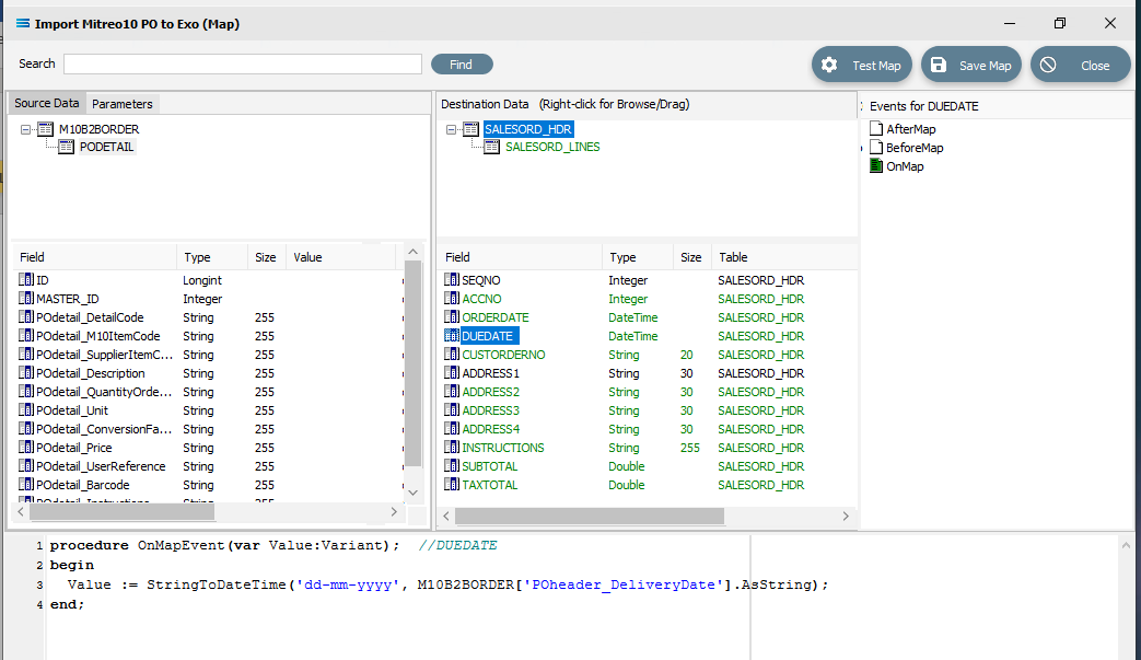
procedure OnMapEvent(var Value:Variant); //DUEDATEbegin Value := StringToDateTime('dd-mmm-yyyy', M10B2BORDER['POheader_DeliveryDate’].AsString);end;When you click out of the Scripting Area, if you are prompted to save your changes, click Yes. This field should now display in GREEN.
Make sure that when you amend this code that you use the correct type of quote marks, else the script will not compile. The quote marks should be single and vertically straight such as '.
To facilitate the orders totals mapping, a running order total calculation needs to be added as an AfterMap event on the SALESORD_LINES dataset. This introduces two new concepts: variables and logging. Firstly, the total for the current line is calculated and stored in the local variable vLineValue, which exists only within the event script. It is then added to the running total stored in the variable Global1, which is accessible in all event scripts in the Map. The results of the calculations from these two variables are output to the log.
Click on SALESORD_LINES to make that dataset the current active dataset. Click on the AfterMap icon in the Events for SALESORD_LINES pane. Click your cursor anywhere within the Scripting Area, and the following code should appear.
procedure AfterMapEvent(var Value:Variant); //SALESORD_LINESbegin // The AfterMap event will fire even for records that are skipped by setting Value:=False // in the BeforeMap. To run AfterMap code only for records that were not skipped wrap your // code with the following commented check // if Value then // Begin //End; Value := end;Change the code to the following. If you prefer, you can leave the lines that are pre-fixed by two diagonal lines // because they are just comments. But for tidiness in this tutorial, they are removed or replaced.
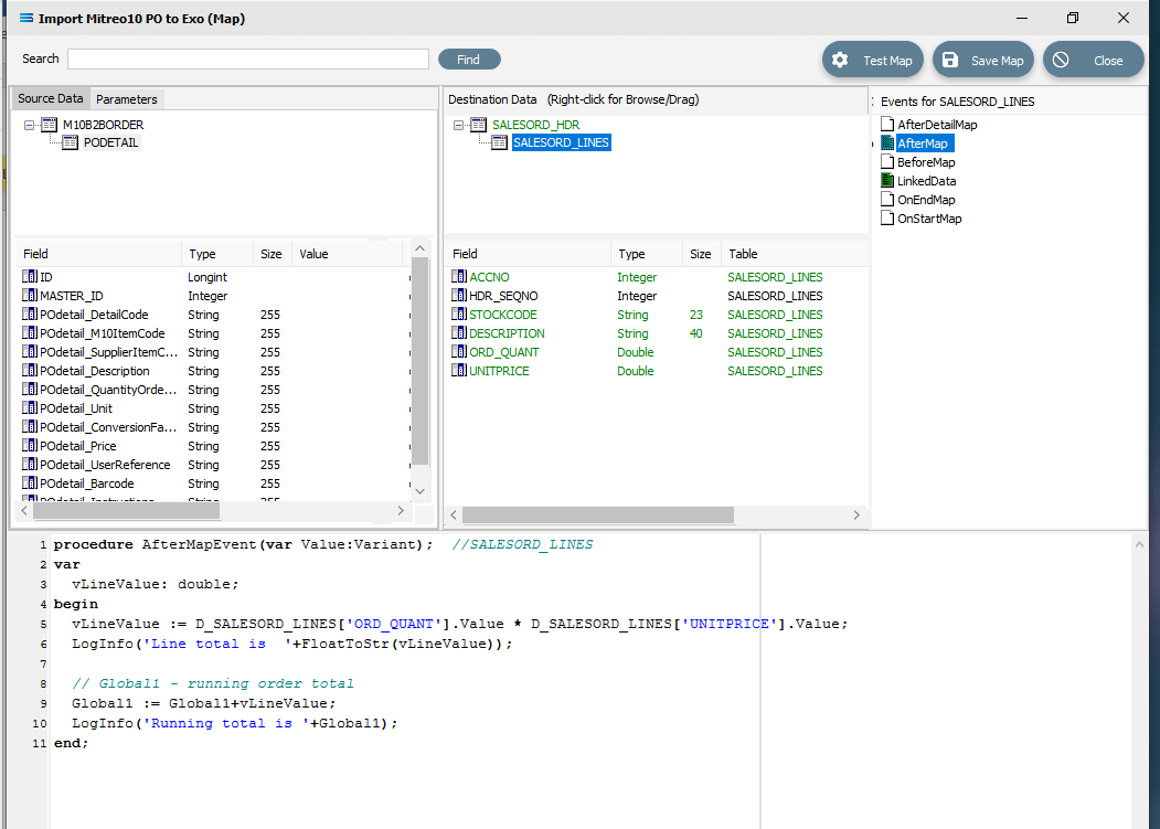
procedure AfterMapEvent(var Value:Variant); //SALESORD_LINESvar vLineValue: double;begin vLineValue := D_SALESORD_LINES['ORD_QUANT'].Value * D_SALESORD_LINES['UNITPRICE'].Value; LogInfo('Line total is '+FloatToStr(vLineValue)); // Global1 – running order total Global1 := Global1+vLineValue; LogInfo('Running total is '+Global1);end;Make sure that your lines of code do not wrap onto a second line because this will affect the way that the script is read and processed. After entering the code as above, right-click in the Scripting Area and select Test Compile to verify that there are no errors and that the code has compiled successfully. Then click on another field name in the Destination Data pane, and if you are prompted to save your changes, click Yes. To see this code, click on the AfterMap icon in the Events for SALESORD_LINES pane.
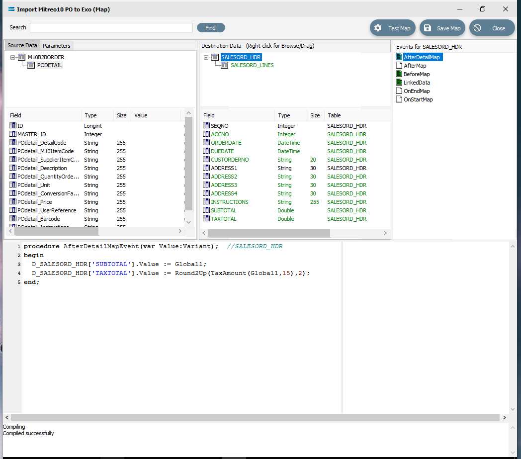
However, just having a total in the variable is not enough. It has to be assigned to a destination field. This is done in the AfterDetailMap event for the SALESORD_HDR dataset. Click on SALESORD_HDR to make that dataset the current active dataset. Click on the AfterDetailMap icon in the Events for SALESORD_HDR pane. Position your cursor in the Scripting Area, and the following code should appear.
procedureAfterDetailMapEvent(varValue:Variant);//SALESORD_HDRbeginValue :=end;Replace this code with the following to assign the values of the variables to the fields in the destination.
procedureAfterDetailMapEvent(varValue:Variant);//SALESORD_HDRbeginD_SALESORD_HDR['SUBTOTAL'].Value := Global1;D_SALESORD_HDR['TAXTOTAL'].Value := Round2Up(TaxAmount(Global1,15),2);end;Again, you can Test Compile to error check your code. A successful compile will change the event icon to GREEN. Click on any field or node name in the Destination Data pane to save your script. Again, when prompted to save the script, reply Yes.
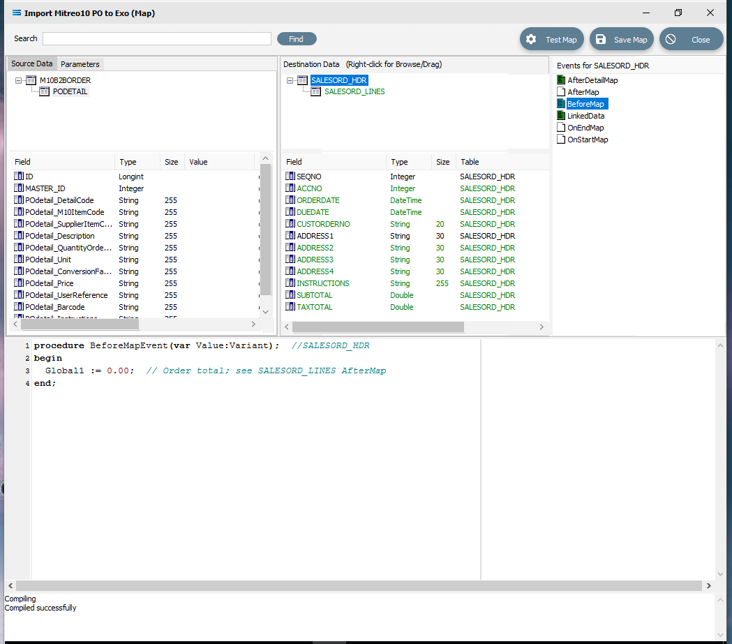
Finally, the running total variable Global1 must be reset to zero for every order that is processed. To do this, code must be entered for a BeforeMap event in the SALESORD_HDR dataset. If not still selected, click on SALESORD_HDR to make the dataset the current active dataset. Click on the BeforeMap icon in the Events for SALESORD_HDR pane. Click into the Scripting Area, and replace the auto‑generated code with the following:
procedureBeforeMapEvent(varValue:Variant);//SALESORD_HDRbeginGlobal1 :=0.00;// Order total; see SALESORD_LINES AfterMapend;The comment after the 2 diagonal slashes on the 3rd line will be read only and will not be processed. Right-click while still in the Scripting Area to Test Compile to error check your code. A successful compile will change the event icon to GREEN. Click on any field or node/table name in the Destination Data pane to save your script. To check the code, you can click on the BeforeMap event icon for the SALESORD_HDR dataset.
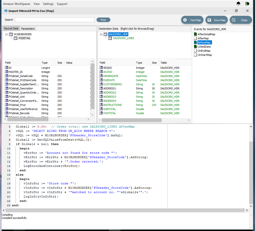
The last field to be still lacking proper mapping is ACCNO in the order header table SALESORD_HDR. The order file does not include the account number from the system that we are importing into, so we need to determine what this number is, based on another key field. In this tutorial, this key field is called POheader_StoreCode. The EXO system into which the data is being imported, stores these codes against the debtor accounts in the BRANCH field. This next step will add the appropriate mapping to determine the value in SALESORD_HDR.ACCNO, and reject the order if the account cannot be found or identified. To make this action possible, additional code needs to be added to the BeforeMap event on SALESORD_HDR – including introduction of another global variable. Click on SALESORD_HDR to make the dataset the current active dataset.
Click on the BeforeMap icon in the Events for SALESORD_HDR pane. The code that you have just edited will display in the Scripting Area. Replace the code with the following code to make a query on the destination database, and then store the returned value in the variable Global2. Then the value of the variable is checked to determine whether to proceed with the order or reject it.
procedureBeforeMapEvent(varValue:Variant);//SALESORD_HDRvarvSQL, vErrStr, vInfoStr:string;beginGlobal1 :=0.00;// Order total; see SALESORD_LINES AfterMapvSQL :='SELECT ACCNO FROM DR_ACCS WHERE BRANCH =';vSQL := vSQL + M10B2BORDER['POheader_StoreCode'].AsSql;Global2 := GetSQLValueFromDest(vSQL,0);ifGlobal2 = nullthenbeginvErrStr :='Account not found for store code "';vErrStr := vErrStr + M10B2BORDER['POheader_StoreCode'].AsString;vErrStr := vErrStr +'".Order rejected.';LogErrorAndContinue(vErrStr);endelsebeginvInfoStr :='Store code "';vInfoStr := vInfoStr + M10B2BORDER['POheader_StoreCode'].AsString;vInfoStr := vInfoStr +'"matched to account no. "'+Global2+'".';LogInfo(vInfoStr);end;end;After entering the code as above, right-click and Test Compile. The message “Compiling” and “Compiled successfully” should appear on separate lines in the messages pane. Correct any error and re-test until the code is accepted.
Then click on any field or table name in the Destination Data pane to save your script. Reply Yes to the prompt to save the script.
You are on the home straight. To complete the mapping, the value of the variable Global2 needs to be assigned to SALESORD_HDR.ACCNO. Ensure that SALESORD_HDR is the current active table. Click on the field ACCNO from the lower Destination Data pane. Replace the code in the Scripting Area with the following:
procedureOnMapEvent(varValue:Variant);//ACCNObeginValue := Global2;// Assigned in the BeforeMapend;The comment on the line will be ignored and not processed. Click on SALESORD_HDR.ACCNO in the Destination Data pane to save the script. Reply Yes when prompted to save the script.
Now save the Map and commit all of the mapping and scripting by clicking Save Map in the top right corner. Select OK to close the successful save message, then click on the Close button to close the map designer Import Mitre10 PO to Exo (Map) window.
To commit all the mapping and scripting, click Save to save and close the mapping module.
The Map named Import Mitre10 PO to Exo will now appear in the structure tree under Configuration > Components > Maps.
Test The Map
Now test the Map to ensure it is working:
Open the Maps module again by clicking on Import Mitre10 PO to Exo, and click on the Design button.
The Map Designer screen called Import Mitre10 PO to Exo will display, with only the Source data M10B2BORDER showing, and SALESORD_HDR showing under Destination Data. SALESORD_HDR will be displayed in GREEN.
Make sure that the file specified in the File Connection called Mitre10: Purchase Order has been copied correctly and is available in the directory.
As a quick check, if the required file is not present in the selected directory then there will be no entries in the Value column of the POdetail table in the Source pane.
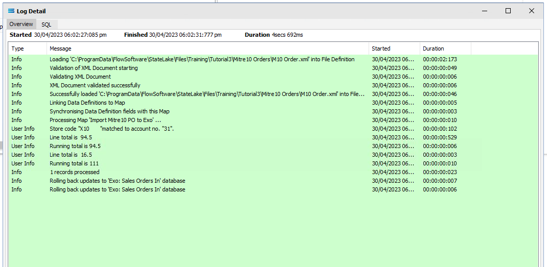
Click Test Map in the top right corner of the screen, to execute the Map in memory and generate a processing log which is then presented in a preview pane. If there is no data selected, then the Log will have a pale YELLOW background. If this occurs check your definitions, change whatever is incorrect, and try the test again. Outright errors will have a dark PINK background, but with a successful test, the background will be pale GREEN. Examples of these log file colours are below.
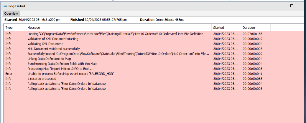
If you are testing the Map (or in due course running the associated Action) and encounter an error that produces a PINK Log file, make sure to carefully read the details about how the error was produced. This tutorial has one file that has intentionally been set up to fail, so depending on which file you are processing, this file may be the cause of the error. The error message that is generated in this case, was entered as part of a BeforeMap event on SALESORD_HDR starting at item #27 in the previous section.
Close the pop-up preview of the log and the DB Definition window for Exo: Sales Orders In will be open.
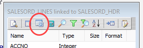
The query SALESORD_HDR and SALESORD_LINES linked to SALESORD_HDR will be displayed on the canvas. Click on the Preview button on SALESORD_HDR to view the processed records.
Using the X in the upper right corner, close the Preview Data pane, or click OK.
Click on the Preview button on SALESORD_LINES linked to SALESORD_HDR to view the processed records.
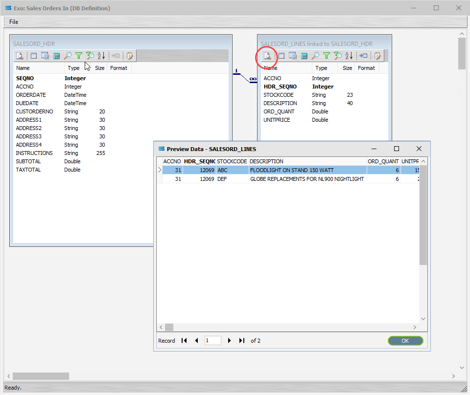
Using the X in the upper right corner, close the Preview Data pane, or click OK.
Select File Close on the canvas, the Close button on the Map Designer screen, and the Cancel button on the Import Mitre10 PO to Exo data entry window.
The Map has now been configured to insert records into a two-level table structure from a multi-tier XML source file. The links have been tested in memory to ensure that the Map has all the information required for a successful extraction.
However, no actual file to database activity has been generated.
The next step pulls all the configured components together to produce the destination tables.
What Action To Take - Creating An Action
The final step is to pull all the definitions and configured components together to form an executable process to produce the destination database. This process is called an Action. While the details for an Action can be created manually, Statelake can also generate the Action quickly and easily for you.
Designer will already be open. If not, open the Statelake module Designer for the selected configuration called Statelake_Training. An expanded structure tree is displayed on the left side of the screen.
Create The Action Automatically
Follow the path Configuration > Components > Maps. Right‑click on the Map you have just created Import Mitre10 PO to Exo, and choose Create Action from the drop‑down list. All the relevant components will be automatically added to this Action.
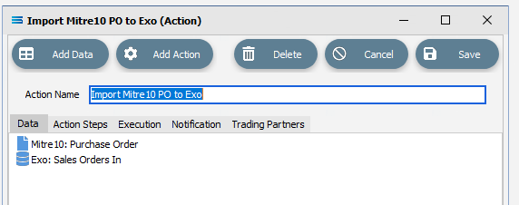
There is no need to do anything with this window, except select Save on the top right corner to close the module.
The Action named Import Mitre10 PO to Exo will now appear in the structure tree under Configuration > Actions.
Run The Action
To run this Action, under the Actions directory, right-click on the Import Mitre10 PO to Exo, then select Run Action from the available options.
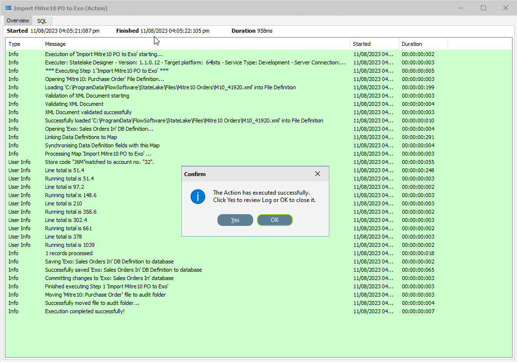
A window will pop-up showing the processing steps in a preview log, that will show the steps that were completed, how many records were extracted and processed, and where the destination file was saved. When the Action has been completed a status message will pop-up on screen indicating that processing is complete, and advising whether the process was successful or an error was encountered.
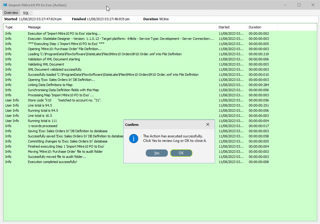
A successful Action will offer two choices – click Yes to review the log, or click OK to close the log without review. To close the Log after review, click the X in the upper right corner.
Logs can be re-opened at any stage, as many times as required. To review a Log from the Manage Logs window, double-click on the Log required. To drill into any line of the Log, double-click on the line to see more detail.
The process is now complete, all modules have been closed, and the structure tree will be the only item on the Designer screen.
This Action will process a single file at a time. This is the default behaviour. The source location started with three (3) .xml files.
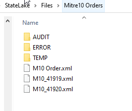
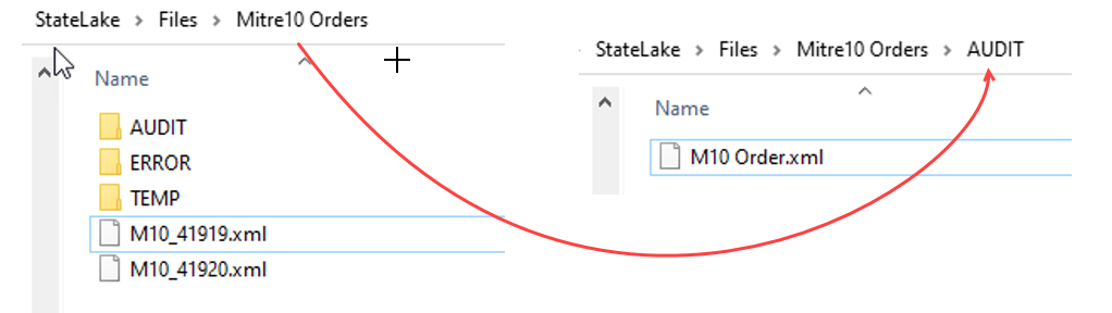
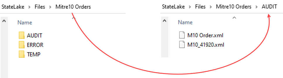
You will have seen from the Log that once this Action has 'been successfully processed, the file that was loaded and processed during the Action called file M10 Order.xml will have been moved into the AUDIT sub directory.
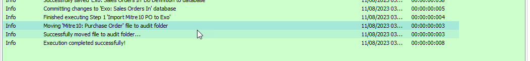
So it will no longer be located in its original sub-directory, as below. It has been moved from Mitre10 Orders to AUDIT so that it does not get re-processed.
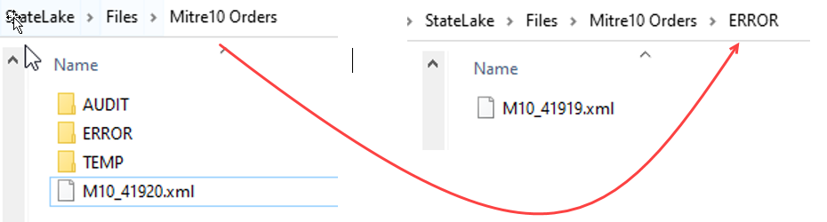
To process another file in the specified sub-directory whose name also fits the selection criteria, re-run the Action by right-click on the Import Mitre10 PO to Exo, then select Run Action from the available options. This time, the Action will encounter an error. This is by design.
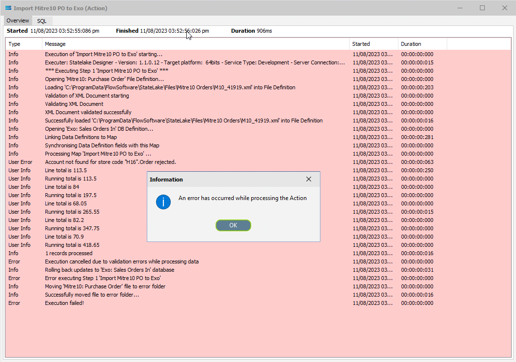
Because of this error, the file that was loaded and processed called M10_41919.xml has been removed from its original location and moved into the ERROR directory.
Click OK to close the dialog box and return to the Log window. Close this window using the X in the upper right corner.
Now run the Action again. This time, the file M10_41920.xml has been successfully processed.
And subsequently moved from its original location into the AUDIT sub-directory, joining the initial file M10 Orders.xml. The original location of Mitre10 Orders now contains no files.
Close the Log window with OK.
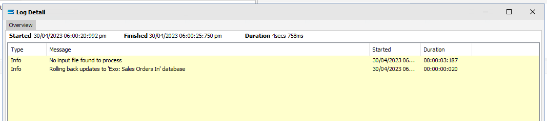
Now, try running the Action one more time. This time the Log displays an unsuccessful completion - otherwise called an Action cancellation.
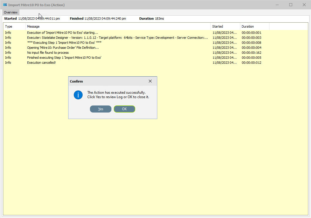
This is because there were no more files in the source location that met the selection criteria specified in the original location.
Summary
Congratulations! You can breathe again - all the hard work is done for this tutorial. A two-level database table has now been generated from a multi-tier XML source file. And you have proven your skills as a fully-fledged scripting ninja.
In summary these are things that have been achieved for this configuration in this tutorial:
An XML file definition has been configured to enable reading of the XML file.
A database definition has been configured to enable writing into related database tables.
Various events have been introduced during mapping.
The use of variables in the mapping script.
Data conversion during scripting.
Querying databases from the map during processing.
Quick Recap Quiz
This has been the biggest and most complicated tutorial so far, with much to take in. Here is a quick quiz to test your knowledge!
In which module would you find the Query Designer?
a. File Definition b. DB Definition c. Action
2. How do XML files differ from flat files?
a. Contain extra information b. They are smaller c. Can be harder to read
3. Which module allows you to transform source data to a different output format?
a. Action b. File Definition c. Map.
4. Which event will be processed first?
a. AfterMap b. OnEndMap c. BeforeMap
5. What does the acronym EDI stand for?
a. Electronic Data Interchange. b. Electronic Detail Input c. Eloise Does Indiana
6. In the Query Designer, are you able to sort the names of the available fields?
a. Only in descending order b. Yes, fully c No, not at all
7. In a database table, what does the foreign key link to?
a. A field in a different table b. An overseas database c. A record in a file
8. What type of associate file does an XML file always need to have for a File Definition?
a. Executable b. Schema c. MS SQL
9. Which type of variable allows a value to be used anywhere across a configuration?
a. Local global b. Script variable c. Super global
10. This data segment is most likely to have come from which file type?
<OrderLine> <LineNumber>1</LineNumber> <ProductCode>AnythingYouFancy</ProductCode> <PackSize>2</PackSize> <OrderQuantity>10</OrderQuantity> <Colour>Sparkly</Colour> </OrderLine>a. XML b. DAT c. CSV
Next Steps
You are now becoming more familiar with the processes involved in manipulating your data, and more familiar with the ease with which files and databases are handled by Statelake.
The last step on this journey brings together all of the things you have learnt so far, and introduces some new and exciting functions:
Tutorial 4 - Extracting XML Invoices Out Of A Database
Tutorial 5 - Statelake Magic SQL
Tutorial 6 - Import CSV Purchase Orders Into A Database
Tutorial 7 - Exporting And Importing Configuration Data
Quick recap quiz answers
b 2. a 3. c 4. c 5. a 6. b 7. a 8. b 9. c 10. a
Congratulations on your progress!